I want to talk about a comonad that came up at work the other day. Actually, two of them, as the data structure in question is a comonad in at least two ways, and the issue that came up is related to the difference between those two comonads.

This post is sort of a continuation of the Comonad Tutorial, and we can call this “part 3”. I’m going to assume the reader has a basic familiarity with comonads.

Inductive Graphs

At work, we develop and use a Scala library called Quiver for working with graphs). In this library, a graph is a recursively defined immutable data structure. A graph, with node IDs of type V, node labels N, and edge labels E, is constructed in one of two ways. It can be empty:

1

def empty[V,N,E]: Graph[V,N,E]

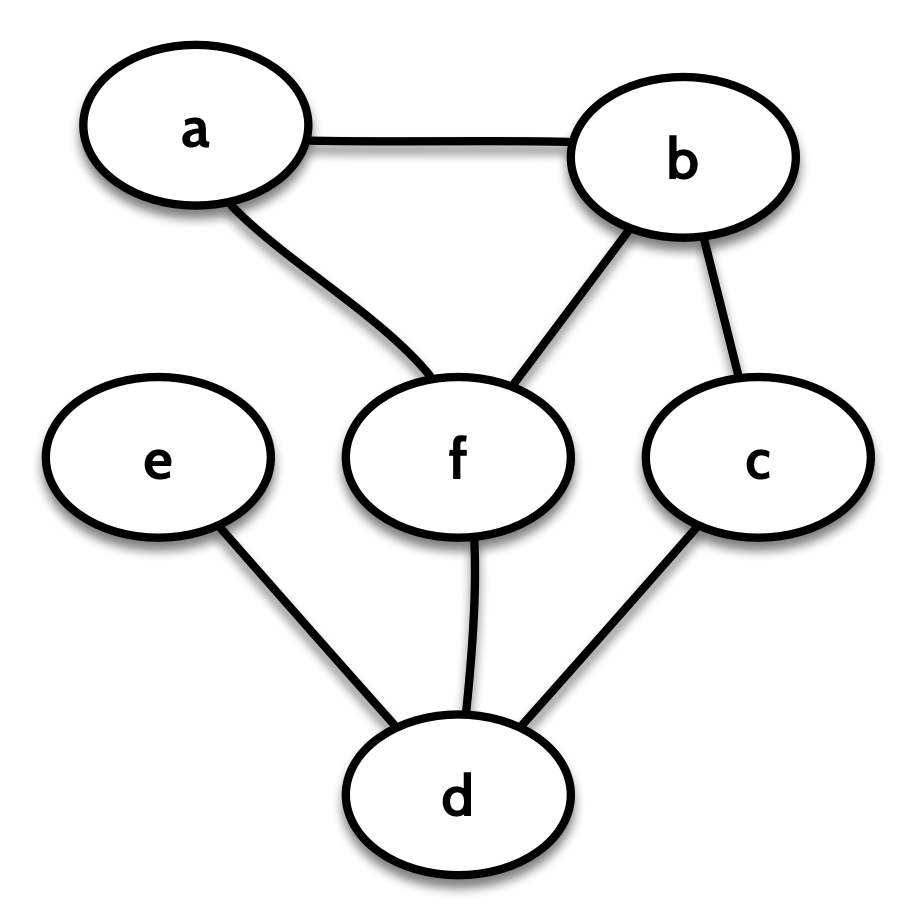
Or it can be of the form c & g, where c is the context of one node of the graph and g is the rest of the graph with that node removed:

1
2
3
4
5
6
7
8

case class Context[V,N,E](
  inEdges: Vector[(E,V)],
  vertex: V,
  label: N,
  outEdges: Vector[(E,V)]
) {
  def &(g: Graph[V,N,E]): Graph[V,N,E] = ???
}

By the same token, we can decompose a graph on a particular node:

1
2
3
4

g: Graph[V,N,E]
v: V

g decomp v: Option[GDecomp[V,N,E]]

Where a GDecomp is a Context for the node v (if it exists in the graph) together with the rest of the graph:

1

case class GDecomp[V,N,E](ctx: Context[V,N,E], rest: Graph[V,N,E])

Recursive decomposition

Let’s say we start with a graph g, like this:

I’m using an undirected graph here for simplification. An undirected graph is one in which the edges don’t have a direction. In Quiver, this is represented as a graph where the “in” edges of each node are the same as its “out” edges.

If we decompose on the node a, we get a view of the graph from the perspective of a. That is, we’ll have a Context letting us look at the label, vertex ID, and edges to and from a, and we’ll also have the remainder of the graph, with the node a “broken off”:

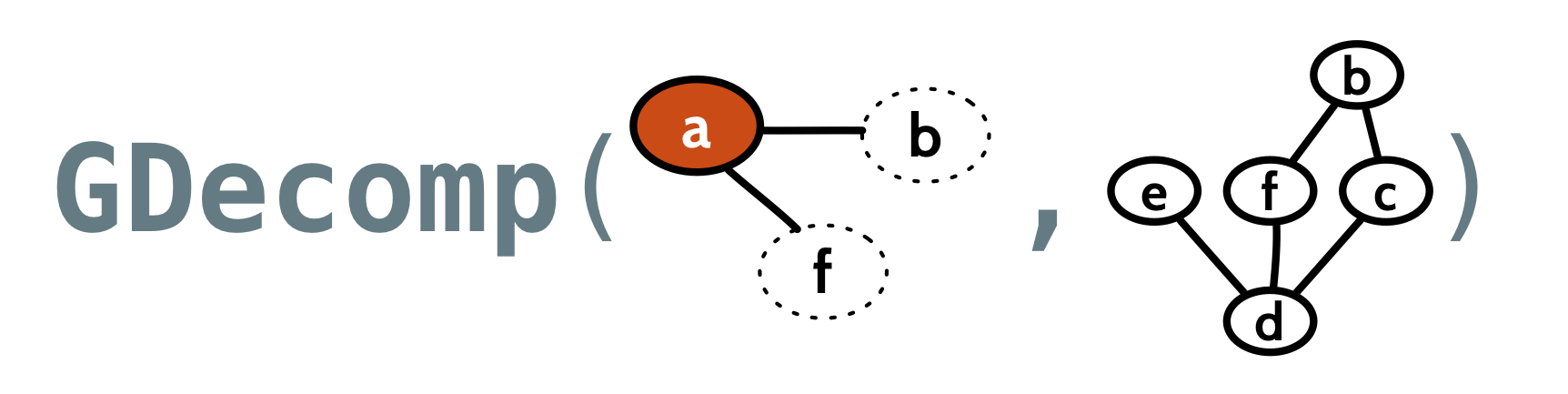
Quiver can arbitrarily choose a node for us, so we can look at the context of some “first” node:

1
2
3

g: Graph[V,N,E]

g.decompAny: Option[GDecomp[V,N,E]]

We can keep decomposing the remainder recursively, to perform an arbitrary calculation over the entire graph:

1
2
3
4

f: (Context[V,N,E], B) => B
b: B

(g fold b)(f): B

The implementation of fold will be something like:

1
2
3

g.decompAny map {
  case GDecomp(ctx, rest) => f(ctx, rest.fold(b)(f))
} getOrElse b

For instance, if we wanted to count the edges in the graph g, we could do:

1
2
3

(g fold 0) {
  case (Context(ins, _, _, outs), b) => ins.size + outs.size + b
}

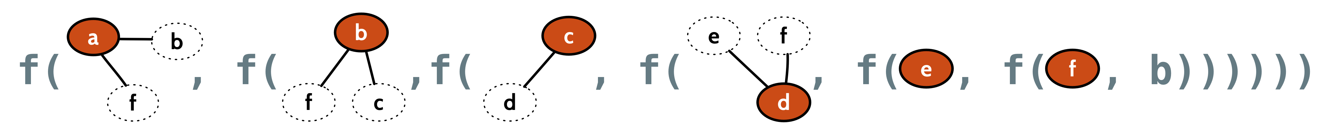
The recursive decomposition will guarantee that our function doesn’t see any given edge more than once. For the graph g above, (g fold b)(f) would look something like this:

Graph Rotations

Let’s now say that we wanted to find the maximum degree of a graph. That is, find the highest number of edges to or from any node.

A first stab might be:

1
2
3
4
5

def maxDegree[V,N,E](g: Graph[V,N,E]): Int =
  g.fold(0) {
    case (Context(ins, _, _, outs), z) =>
      (ins.size + outs.size) max z
  }

But that would get the incorrect result. In our graph g above, the nodes b, d, and f have a degree of 3, but this fold would find the highest degree to be 2. The reason is that once our function gets to look at b, its edge to a has already been removed, and once it sees f, it has no edges left to look at.

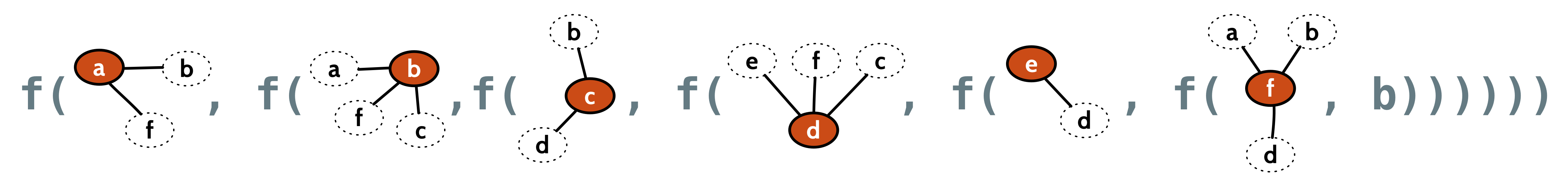
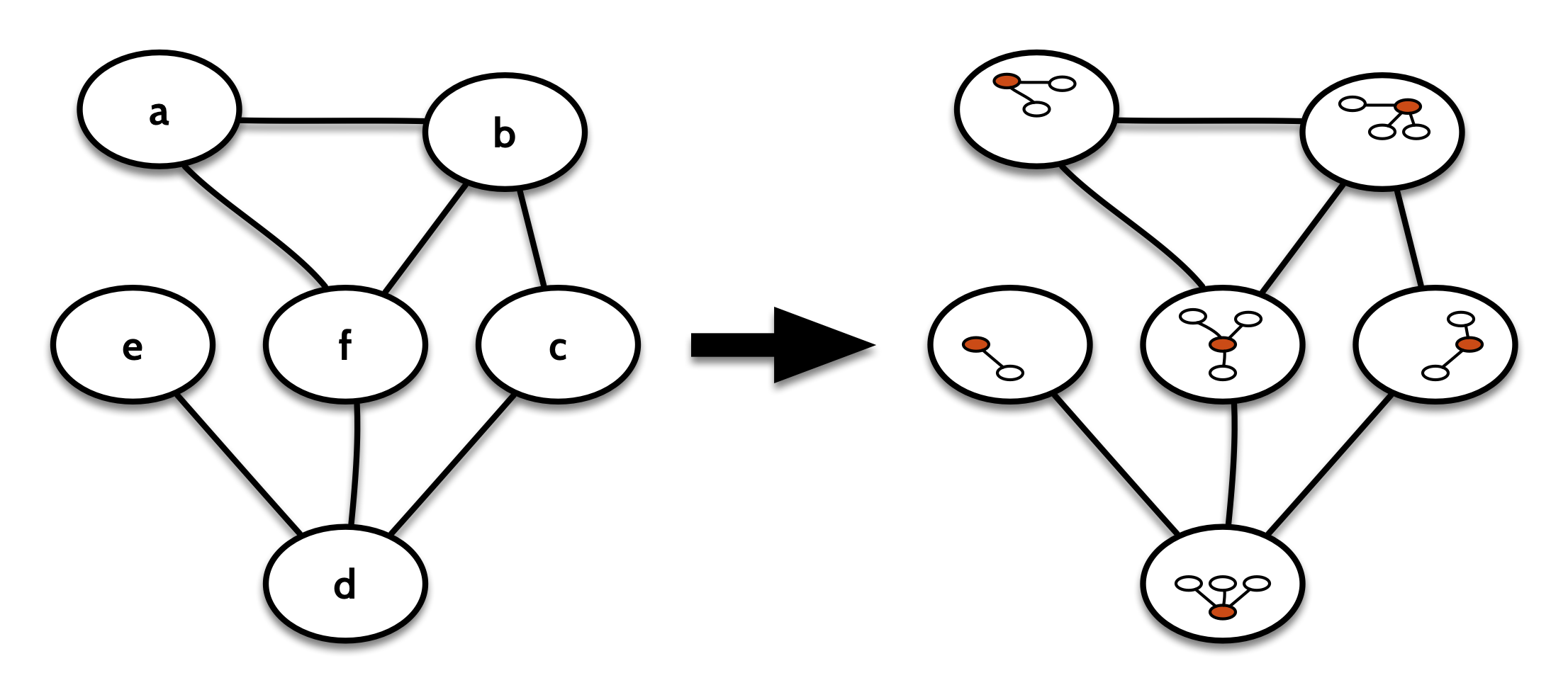
This was the issue that came up at work. This behaviour of fold is both correct and useful, but it can be surprising. What we might expect is that instead of receiving successive decompositions, our function sees “all rotations” of the graph through the decomp operator:

That is, we often want to consider each node in the context of the entire graph we started with. In order to express that with fold, we have to decompose the original graph at each step:

1
2
3
4
5
6
7

def maxDegree[V,N,E](g: Graph[V,N,E]): Int =
  g.fold(0) { (c, z) =>
    g.decompose(c.vertex).map {
      case GDecomp(Context(ins, _, _, outs), _) =>
        ins.size + outs.size
    }.getOrElse(0) max z
  }

But what if we could have a combinator that labels each node with its context?

1

def contextGraph(g: Graph[V,N,E]): Graph[V,Context[V,N,E],E]

Visually, that looks something like this:

If we now fold over contextGraph(g) rather than g, we get to see the whole graph from the perspective of each node in turn. We can then write the maxDegree function like this:

1
2
3
4

def maxDegree[V,N,E](g: Graph[V,N,E]): Int =
  contextGraph(g).fold(0) { (c, z) =>
    z max (c.label.ins.size + c.label.outs.size)
  }

Two different comonads

This all sounds suspiciously like a comonad! Of course, Graph itself is not a comonad, but GDecomp definitely is. The counit just gets the label of the node that’s been decomped out:

1
2
3
4
5
6
7

def gdecompComonad[V,E] = new Comonad[λ[α => GDecomp[V,α,E]]] {

  def counit[A](g: GDecomp[V,A,E]): A = g.ctx.label

  def cobind[A,B](g: GDecomp[V,A,E])(
                  f: GDecomp[V,A,E] => B): GDecomp[B] = ???
}

The cobind can be implemented in one of two ways. There’s the “successive decompositions” version:

1
2
3
4
5
6
7

def cobind[A,B](g: GDecomp[V,A,E])(
                f: GDecomp[V,A,E] => B): GDecomp[B] =
  GDecomp(g.ctx.copy(label = f(g)),
          g.rest.decompAny.map {
            val GDecomp(c, r) = cobind(_)(f)
            c & r
          } getOrElse empty)

Visually, it looks like this:

It exposes the substructure of the graph by storing it in the labels of the nodes. It’s very much like the familiar NonEmptyList comonad, which replaces each element in the list with the whole sublist from that element on.

So this is the comonad of recursive folds over a graph. Really its action is the same as as just fold. It takes a computation on one decomposition of the graph, and extends it to all sub-decompositions.

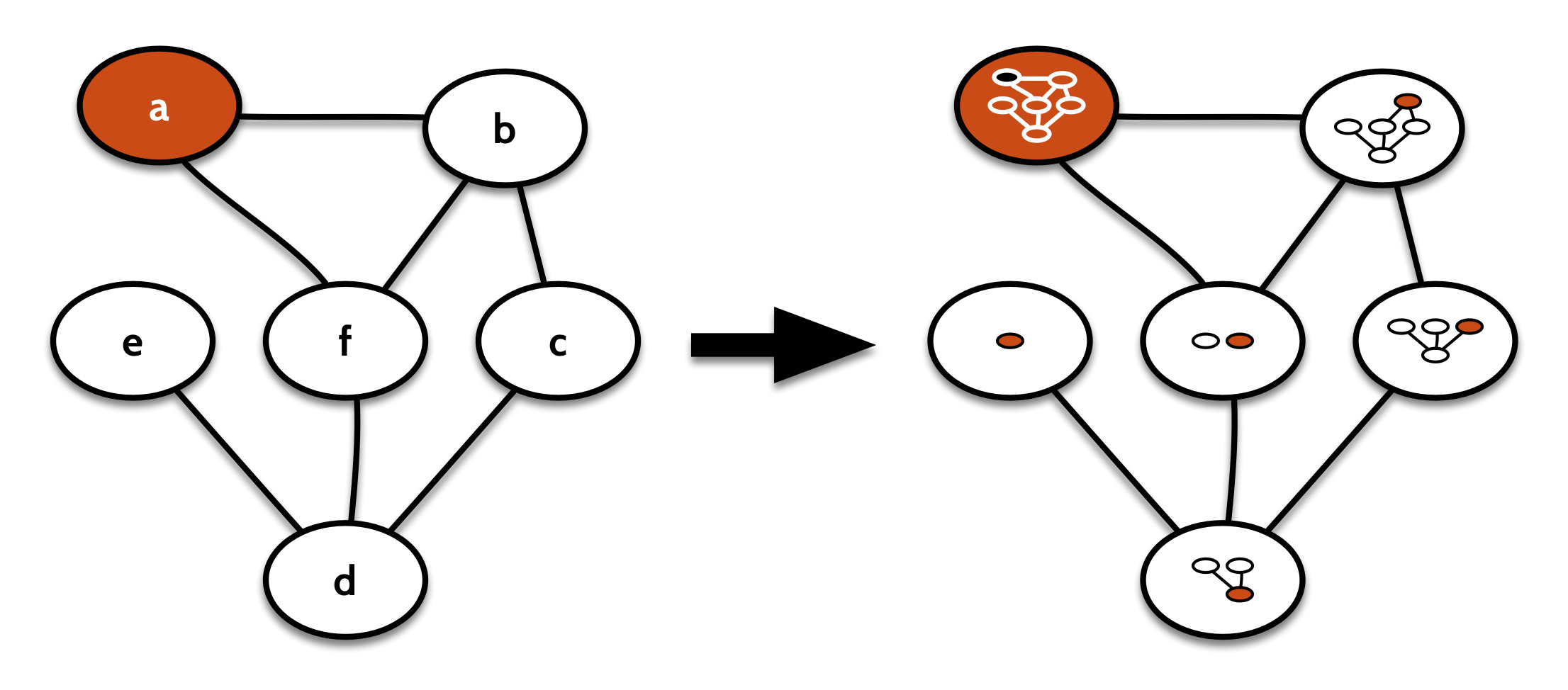
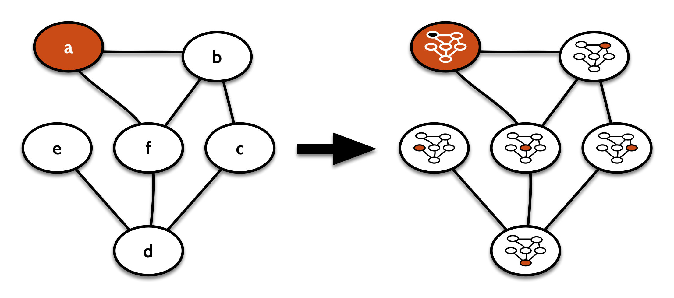
But there’s another, comonad that’s much more useful as a comonad. That’s the comonad that works like contextGraph from before, except instead of copying the context of a node into its label, we copy the whole decomposition; both the context and the remainder of the graph.

That one looks visually more like this:

Its cobind takes a computation focused on one node of the graph (that is, on a GDecomp), repeats that for every other decomposition of the original graph in turn, and stores the results in the respective node labels:

1
2
3
4
5
6
7
8

def cobind[A,B](g: GDecomp[V,A,E])(
                f: GDecomp[V,A,E] => B): GDecomp[B] = {
  val orig = g.ctx & g.rest
  GDecomp(g.ctx.copy(label = f(g)),
          rest.fold(empty) { (c, acc) =>
            c.copy(label = f(orig.decomp(c.vertex).get)) & acc
          })
}

This is useful for algorithms where we want to label every node with some information computed from its neighborhood. For example, some clustering algorithms start by assigning each node its own cluster, then repeatedly joining nodes to the most popular cluster in their immediate neighborhood, until a fixed point is reached.

As a simpler example, we could take the average value for the labels of neighboring nodes, to apply something like a low-pass filter to the whole graph:

1
2
3
4
5
6
7

def lopass[V,E](g: Graph[V,Int,E]): Graph[V,Int,E] =
  g.decompAny.map { d => cobind(d) { x =>
    val neighbors = (x.inEdges ++ x.outEdges).map { n =>
      g.decomp(n).get.ctx.label
    }
    (neighbors.sum + x.label) / (neighbors.length + 1)
  }} getOrElse g

The difference between these two comonad instances is essentially the same as the difference between NonEmptyList and the nonempty list Zipper.

It’s this latter “decomp zipper” comonad that I decided to ultimately include as the Comonad instance for quiver.GDecomp.

I’ve been having fun exploring adjunctions lately and thinking about how we can take a monad apart and compose it the other way to get a comonad, and vice versa. Often I’ll find that a comonad counterpart of a given monad gives an interesting perspective on that monad, and ditto for a monad cousin to a given comonad.

The monad for monoids

Let’s take an example. There is a category of monoids Mon with monoids as objects and monoid homomorphisms as arrows between them. Then there is a functor from Set to Mon that takes any ordinary type A to the free monoid generated by A. This is just the List[A] type together with concatenation as the multiplication and the empty list as the identity element.

This free functor has a right adjoint that takes any monoid M in Mon to its underlying set M. That is, this right adjoint “forgets” that M is a monoid, leaving us with just an ordinary type.

If we compose these two functors, we get a monad. If we start with a type A, get its free monoid (the List[A] monoid), and then go from there to the underlying type of the free monoid, we end up with the type List[A]. The unit of our adjunction is then a function from any given type A to the type List[A].

1

def unit[A](a: A): List[A] = List(a)

Structure ⊣ Interpretation

But then what is the counit? Remember that for any adjunction, we can compose the functors one way to get a monad, and compose them the other way to get a comonad.

In that case we have to start with a monoid M, then “forget”, giving us the plain type M. Then we take the free monoid of that to end up with the List[M] monoid.

But notice that we are now in the monoid category. In that category, List is a comonad. And since we’re in the category of monoids, the counit has to be a monoid homomorphism. It goes from the free monoid List[A] to the monoid A:

1
2

def counit[A:Monoid](as: List[A]): A =
  as.foldRight(Monoid[A].zero)(Monoid[A].append)

If we apply the counit for this comonad to the free monoid, we get the join for our monad:

1

def join[A](as: List[List[A]]): List[A] = counit(as)

And to get the duplicate or extend operation in the comonad, we just turn the crank on the adjunction:

1
2

def duplicate[A](as: List[A]): List[List[A]] =
  as.map(unit(_))

The duplicate just puts each element into its own sublist. With regard to extend, this just means that given any catamorphism on List, we can turn that into a homomorphism on free monoids.

1
2

def extend[A,B](as: List[A])(f: List[A] => B): List[B] =
  as.map(x => f(unit(x)))

All the interesting parts of List are the parts that make it a monoid, and our comonad here is already in a category full of monoids. Therefore the coKleisli composition in this comonad is kind of uninteresting. All it’s saying is that if we can fold a List[A] to a B, and a List[B] to a C, then we can fold a List[A] to a C, by considering each element as a singleton list.

Forget ⊣ Cofree

Let’s now consider another category, call it End(Set), which is the category of endofunctors in Set.

The arrows in this category are natural transformations:

1
2
3

trait ~>[F[_],G[_]] {
  def apply[A](x: F[A]): G[A]
}

There’s another category, Com, which is the category of comonads on Set. The arrows here are comonad homomorphisms. A comonad homomorphism from F to G is a natural transformation f: F ~> G satisfying the homomorphism law:

1

f(x).duplicate == f(x.duplicate) map f

There is a forgetful functor Forget: Com -> End(Set) that takes a comonad to its underlying endofunctor (forgetting that it’s a comonad). And this functor has a right adjoint Cofree: End(Set) -> Com which generates a cofree comonad on a given endofunctor F. This is the following data type:

1

case class Cofree[F[_],A](head: A, tail: F[Cofree[F,A]])

Note that not only is the endofunctor Cofree[F,?] a comonad (in Set) for any functor F, but the higher-order type constructor Cofree is itself is a comonad in the endofunctor category. It’s this latter comonad that is induced by the Forget ⊣ Cofree adjunction. That is, we start at an endofunctor F, then go to comonads via Cofree[F,?], then back to endofunctors via Forget.

The unit for this adjunction is then a comonad homomorphism. Remember, this is the unit for a monad in the category Com of comonads:

1
2
3

def unit[F[_]:Comonad,A](x: F[A]): Cofree[F,A] =
  Cofree(x.counit, x.extend(unit(_)))
}

This will start with a value of type F[A] in the comonad F, and then unfold an F-branching stream from it. Note that the first level of this will have the same structure as x.

If we take unit across to the End(Set) category, we get the duplicate for our comonad:

1
2

def duplicate[F[_],A](c: Cofree[F,A]): Cofree[Cofree[F,?],A] =
  unit(c)

Note that this is not the duplicate for the Cofree[F,?] comonad. It’s the duplicate for Cofree itself which is a comonad in an endofunctor category.

Turning the crank on the adjunction, the counit for this comonad now has to be the inverse of our unit. It takes the heads of all the branches of the given F-branching stream.

1
2
3

def counit[F[_]:Functor,A](c: Cofree[F,A]): F[A] =
  c.tail.map(_.head)
}

Sending that over to the comonad category, we get the join for our monad:

1
2

def join[F[_]:Comonad,A](c: Cofree[Cofree[F,?],A]): Cofree[F,A] =
  counit(c)

In the previous post, we looked at the Reader/Writer monads and comonads, and discussed in general what comonads are and how they relate to monads. This time around, we’re going to look at some more comonads, delve briefly into adjunctions, and try to get some further insight into what it all means.

Nonempty structures

Since a comonad has to have a counit, it must be “pointed” or nonempty in some sense. That is, given a value of type W[A] for some comonad W, we must be able to get a value of type A out.

The identity comonad is a simple example of this. We can always get a value of type A out of Id[A]. A slightly more interesting example is that of non-empty lists:

1

case class NEL[A](head: A, tail: Option[NEL[A]])

So a nonempty list is a value of type A together with either another list or None to mark that the list has terminated. Unlike the traditional List data structure, we can always safely get the head.

But what is the comonadic duplicate operation here? That should allow us to go from NEL[A] to NEL[NEL[A]] in such a way that the comonad laws hold. For nonempty lists, an implementation that satisfies those laws turns out to be:

1
2
3
4
5
6

case class NEL[A](head: A, tail: Option[NEL[A]]) {
  ...
  def tails: NEL[NEL[A]] =
    NEL(this, tail.map(_.tails))
  ...
}

The tails operation returns a list of all the suffixes of the given list. This list of lists is always nonempty, because the first suffix is the list itself. For example, if we have the nonempty list [1,2,3] (to use a more succinct notation), the tails of that will be [[1,2,3], [2,3], [3]]

To get an idea of what this means in the context of a comonadic program, think of this in terms of coKleisli composition, or extend in the comonad:

1
2

  def extend[A,B](f: NEL[A] => B): NEL[B] =
    tails map f

When we map over tails, the function f is going to receive each suffix of the list in turn. We apply f to each of those suffixes and collect the results in a (nonempty) list. So [1,2,3].extend(f) will be [f([1,2,3]), f([2,3]), f([3])].

The name extend refers to the fact that it takes a “local” computation (here a computation that operates on a list) and extends that to a “global” computation (here over all suffixes of the list).

Or consider this class of nonempty trees (often called Rose Trees):

1

case class Tree[A](tip: A, sub: List[Tree[A]])

A tree of this sort has a value of type A at the tip, and a (possibly empty) list of subtrees underneath. One obvious use case is something like a directory structure, where each tip is a directory and the corresponding sub is its subdirectories.

This is also a comonad. The counit is obvious, we just get the tip. And here’s a duplicate for this structure:

1
2

  def duplicate: Tree[Tree[A]] =
    Tree(this, sub.map(_.duplicate))

Now, this obviously gives us a tree of trees, but what is the structure of that tree? It will be a tree of all the subtrees. The tip will be this tree, and the tip of each proper subtree under it will be the entire subtree at the corresponding point in the original tree.

That is, when we say t.duplicate.map(f) (or equivalently t extend f), our f will receive each subtree of t in turn and perform some calculation over that entire subtree. The result of the whole expression t extend f will be a tree mirroring the structure of t, except each node will contain f applied to the corresponding subtree of t.

To carry on with our directory example, we can imagine wanting a detailed space usage summary of a directory structure, with the size of the whole tree at the tip and the size of each subdirectory underneath as tips of the subtrees, and so on. Then d extend size creates the tree of sizes of recursive subdirectories of d.

The cofree comonad

You may have noticed that the implementations of duplicate for rose trees and tails for nonempty lists were basically identical. The only difference is that one is mapping over a List and the other is mapping over an Option. We can actually abstract that out and get a comonad for any functor F:

1
2
3
4

case class Cofree[F[_],A](counit: A, sub: F[Cofree[F,A]]) {
  def duplicate(implicit F: Functor[F]): Cofree[F,Cofree[F,A]] =
    Cofree(this, F.map(sub)(_.duplicate))
}

A really common kind of structure is something like the type Cofree[Map[K,?],A] of trees where the counit is some kind of summary and each key of type K in the Map of subtrees corresponds to some drilldown for more detail. This kind of thing appears in portfolio management applications, for example.

Compare this structure with the free monad:

1
2
3

sealed trait Free[F[_],A]
case class Return[F[_],A](a: A) extends Free[F,A]
case class Suspend[F[_],A](s: F[Free[F,A]]) extends Free[F,A]

While the free monad is either an A or a recursive step suspended in an F, the cofree comonad is both an A and a recursive step suspended in an F. They really are duals of each other in the sense that the monad is a coproduct and the comonad is a product.

Comparing comonads to monads (again)

Given this difference, we can make some statements about what it means:

• Free[F,A] is a type of “leafy tree” that branches according to F, with values of type A at the leaves, while Cofree[F,A] is a type of “node-valued tree” that branches according to F with values of type A at the nodes.
• If Exp defines the structure of some expression language, then Free[Exp,A] is the type of abstract syntax trees for that language, with free variables of type A, and monadic bind literally binds expressions to those variables. Dually, Cofree[Exp,A] is the type of closed exresspions whose subexpressions are annotated with values of type A, and comonadic extend reannotates the tree. For example, if you have a type inferencer infer, then e extend infer will annotate each subexpression of e with its inferred type.

This comparison of Free and Cofree actually says something about monads and comonads in general:

• All monads can model some kind of leafy tree structure, and all comonads can be modeled by some kind of node-valued tree structure.
• In a monad M, if f: A => M[B], then xs map f allows us to take the values at the leaves (a:A) of a monadic structure xs and substitute an entire structure (f(a)) for each value. A subsequent join then renormalizes the structure, eliminating the “seams” around our newly added substructures. In a comonad W, xs.duplicate denormalizes, or exposes the substructure of xs:W[A] to yield W[W[A]]. Then we can map a function f: W[A] => B over that to get a B for each part of the substructure and redecorate the original structure with those values. (See Uustalu and Vene’s excellent paper The Dual of Substitution is Redecoration for more on this connection.)
• A monad defines a class of programs whose subexpressions are incrementally generated from the outputs of previous expressions. A comonad defines a class of programs that incrementally generate output from the substructure of previous expressions.
• A monad adds structure by consuming values. A comonad adds values by consuming structure.

The relationship between Reader and Coreader

If we look at a Kleisli arrow in the Reader[R,?] comonad, it looks like A => Reader[R,B], or expanded out: A => R => B. If we uncurry that, we get (A, R) => B, and we can go back to the original by currying again. But notice that a value of type (A, R) => B is a coKleisli arrow in the Coreader comonad! Remember that Coreader[R,A] is really a pair (A, R).

So the answer to the question of how Reader and Coreader are related is that there is a one-to-one correspondence between a Kleisli arrow in the Reader monad and a coKleisli arrow in the Coreader comonad. More precisely, the Kleisli category for Reader[R,?] is isomorphic to the coKleisli category for Coreader[R,?]. This isomorphism is witnessed by currying and uncurrying.

In general, if we have an isomorphism between arrows like this, we have what’s called an adjunction:

1
2
3
4

trait Adjunction[F[_],G[_]] {
  def left[A,B](f: F[A] => B): A => G[B]
  def right[A,B](f: A => G[B]): F[A] => B
}

In an Adjunction[F,G], we say that F is left adjoint to G, often expressed with the notation F ⊣ G.

We can clearly make an Adjunction for Coreader[R,?] and Reader[R,?] by using curry and uncurry:

1
2
3
4
5
6

def homSetAdj[R] = new Adjunction[(?, R), R => ?] {
  def left[A,B](f: ((A, R)) => B): A => R => B =
    Function.untupled(f).curried
  def right[A,B](f: A => R => B): ((A, R)) => B =
    Function.uncurried(f).tupled
}

The additional tupled and untupled come from the unfortunate fact that I’ve chosen Scala notation here and Scala differentiates between functions of two arguments and functions of one argument that happens to be a pair.

So a more succinct description of this relationship is that Coreader is left adjoint to Reader.

Generally the left adjoint functor adds structure, or is some kind of “producer”, while the right adjoint functor removes (or “forgets”) structure, or is some kind of “consumer”.

Composing adjoint functors

An interesting thing about adjunctions is that if you have an adjoint pair of functors F ⊣ G, then F[G[?]] always forms a comonad, and G[F[?]] always forms a monad, in a completely canonical and amazing way:

1
2
3
4
5
6
7
8
9
10
11
12
13
14
15

def monad[F[_],G[_]](A: Adjunction[F,G])(implicit G: Functor[G]) =
  new Monad[λ[α => G[F[α]]]] {
    def unit[A](a: => A): G[F[A]] =
      A.left(identity[F[A]])(a)
    def bind[A,B](a: G[F[A]])(f: A => G[F[B]]): G[F[B]] =
      G.map(a)(A.right(f))
  }

def comonad[F[_],G[_]](A: Adjunction[F,G])(implicit F: Functor[F]) =
  new Comonad[λ[α => F[G[α]]]] {
    def counit[A](a: F[G[A]]): A =
      A.right(identity[G[A]])(a)
    def extend[A,B](a: F[G[A]])(f: F[G[A]] => B): F[G[B]] =
      F.map(a)(A.left(f))
  }

Note that this says something about monads and comonads. Since the left adjoint F is a producer and the right adjoint G is a consumer, a monad always consumes and then produces, while a comonad always produces and then consumes.

Now, if we compose Reader and Coreader, which monad do we get?

1
2

scala> def M[S] = monad(homSetAdj[S])
M: [S]=> scalaz.Monad[[α]S => (α, S)]

That’s the State[S,?] monad!

Now if we compose it the other way, we should get a comonad:

1
2

scala> def W[S] = comonad(homSetAdj[S])
W: [S]=> scalaz.Comonad[[α](S => α, S)]

What is that? It’s the Store[S,?] comonad:

1
2
3
4
5
6
7
8
9
10
11

case class Store[S,A](peek: S => A, cursor: S) {
  def extract: A = peek(cursor)
  def extend[B](f: Store[S,A] => B): Store[S, B] =
    Store(s => f(Store(peek, s)), cursor)
  def duplicate: Store[S, Store[S,A]] =
    extend(identity)
  def map[B](f: A => B): Store[S,B] =
    extend(s => f(s.extract))

  def seek(s: S) = duplicate.peek(s)
}

This models a “store” of values of type A indexed by the type S. We have the ability to directly access the A value under a given S using peek, and there is a distinguished cursor or current position. The comonadic extract just reads the value under the cursor, and duplicate gives us a whole store full of stores such that if we peek at any one of them, we get a Store whose cursor is set to the given s. We’re defining a seek(s) operation that moves the cursor to a given position s by taking advantage of duplicate.

A use case for this kind of structure might be something like image processing or cellular automata, where S might be coordinates into some kind of space (like a two-dimensional image). Then extend takes a local computation at the cursor and extends it to every point in the space. For example, if we have an operation average that peeks at the cursor’s immediate neighbors and averages them, then we can apply a low-pass filter to the whole image with image.extend(average).

The type A => Store[S,B] is also one possible representation of a Lens. I might talk about lenses and zippers in a future post.

In writing up part 2 of my Scala Comonad Tutorial, and coming up with my talk for Scala World, I idly pondered this question:

If all monads are given by composing adjoint pairs of functors, what adjoint pair of functors forms the `Reader` monad? And if we compose those functors the other way, which comonad do we get?

Shachaf Ben-Kiki pointed out on IRC that there are at least two ways of doing this. One is via the Kleisli construction and the other is via the Eilenberg-Moore construction. Dr Eugenia Cheng has a fantastic set of videos explaining these constructions. She talks about how for any monad T there is a whole category Adj(T) of adjunctions that give rise to T (with categories as objects and adjoint pairs of functors as the arrows), and the Kleisli category is the initial object in this category while the Eilenberg-Moore category is the terminal object.

So then, searching around for an answer to what exactly the Eilenberg-Moore category for the R => ? monad looks like (I think it’s just values of type R and functions between them), I came across this Mathematics Stack Exchange question, whose answer more or less directly addresses my original question above. The adjunction is a little more difficult to see than the initial/terminal ones, but it’s somewhat interesting, and what follows is an outline of how I convinced myself that it works.

The adjoint pair

Let’s consider the reader monad R => ?, which allows us to read a context of type R.

The first category involved is Set (or Hask, or Scala). This is just the familiar category where the objects are types (A,B,C, etc.) and the arrows are functions.

The other category is Set/R, which is the slice category of Set over the type R. This is a category whose objects are functions to R. So an object x in this category is given by a type A together with a function of type A => R. An arrow from x: A => R to y: B => R is given by a function f: A => B such that y(f(a)) = x(a) for all a:A.

The left adjoint is R*, a functor from Set to Set/R. This functor sends each type A to the function (p:(R,A)) => p._1, having type (R,A) => R.

1

def rStar[A]: (R,A) => R = _._1

The right adjoint is Π_R, a functor from Set/R to Set. This functor sends each object q: A => R in Set/R to the set of functions R => A for which q is an inverse. This is actually a dependent type inhabited by functions p: R => A which satisfy the identity q(p(a)) = a for all a:A.

Constructing the monad

The monad is not exactly easy to see, but if everything has gone right, we should get the R => ? reader monad by composing Π_R with R*.

We start with a type A. Then we do R*, which gives us the object rStar[A] in the slice category, which you will recall is just _._1 of type (R,A) => R. Then we go back to types via Π_R(rStar[A]) which gives us a dependent type P inhabited by functions p: R => (R,A). Now, this looks a lot like an action in the State monad. But it’s not. These p must satisfy the property that _1 is their inverse. Which means that the R they return must be exactly the R they were given. So it’s like a State action that is read only. We can therefore simplify this to the ordinary (non-dependent) type R => A. And now we have our Reader monad.

Constructing the comonad

But what about the other way around? What is the comonad constructed by composing R* with Π_R? Well, since we end up in the slice category, our comonad is actually in that category rather than in Set.

We start with an object q: A => R in the slice category. Then we go to types by doing Π_R(q). This gives us a dependent type P_A which is inhabited by all p: R => A such that q is their inverse. Then we take rStar[Π_R(q)] to go back to the slice category and we find ourselves at an object f: (R, Π_R(q)) => R, which you’ll recall is implemented as _._1. As an endofunctor in Set/R, λq. rStar[Π_R(q)] takes all q: A => R to p: (R, R => A) => R = _._1 such that p is only defined on R => A arguments whose inverse is q.

That is, the counit for this comonad on elements y: A => R must be a function counit: (R, Π_R(y)) => A such that for _._1: (R, Π_R(y)) => R, the property y compose counit = _._1 holds. Note that this means that the R returned by _._1 and the R returned by y must be the same. Recall that _._1 always returns the first element of its argument, and also recall that the functions in Π_R(y) must have y as their inverse, so they’re only defined at the first element of the argument to _._1. That is p._2(x) is only defined when x = p._1.

If we try to encode that in Scala (ignoring all the “such that”), we get something like:

1
2

def counit[A](p: (R, R => A)): A =
  p._2(p._1)

This looks a lot like a counit for the Store comonad! Except what we constructed is not that. Because of the additional requirements imposed by our functors and by the slice category, the second element of p can only take an argument that is exactly the first element of p. So we can simplify that to (R, () => A) or just (R, A). And we now have the familiar Coreader comonad.

In chapter 11 of our book, we talk about monads in Scala. This finally names a pattern that the reader has seen throughout the book and gives it a formal structure. We also give some intuition for what it means for something to be a monad. Once you have this concept, you start recognizing it everywhere in the daily business of programming.

Today I want to talk about comonads, which are the dual of monads. The utility of comonads in everyday life is not quite as immediately obvious as that of monads, but they definitely come in handy sometimes. Particularly in applications like image processing and scientific computation.

A monad, upside-down

Let’s remind ourselves of what a monad is. A monad is a functor, which just means it has a map method:

1
2
3

trait Functor[F[_]] {
  def map[A,B](x: F[A])(f: A => B): F[B]
}

This has to satisfy the law that map(x)(a => a) == x, i.e. that mapping the identity function over our functor is a no-op.

Monads

A monad is a functor M equipped with two additional polymorphic functions; One from A to M[A] and one from M[M[A]] to M[A].

1
2
3
4

trait Monad[M[_]] extends Functor[M] {
  def unit[A](a: A): M[A]
  def join[A](mma: M[M[A]]): M[A]
}

Recall that join has to satisfy associativity, and unit has to be an identity for join.

In Scala a monad is often stated in terms of flatMap, which is map followed by join. But I find this formulation easier to explain.

Every monad has the above operations, the so-called proper morphisms of a monad, and may also bring to the table some nonproper morphisms which give the specific monad some additional capabilities.

Reader monad

For example, the Reader monad brings the ability to ask for a value:

1
2
3

case class Reader[R,A](run: R => A)

def ask[R]: Reader[R,R] = Reader(r => r)

The meaning of join in the reader monad is to pass the same context of type R to both the outer scope and the inner scope:

1
2

def join[R,A](r: Reader[R,Reader[R,A]]) =
  Reader((c:R) => r.run(c).run(c))

Writer monad

The Writer monad has the ability to write a value on the side:

1
2
3

case class Writer[W,A](value: A, log: W)

def tell[W,A](w: W): Writer[W,Unit] = Writer((), w)

The meaning of join in the writer monad is to concatenate the “log” of written values using the monoid for W (this is using the Monoid class from Scalaz):

1
2

def join[W:Monoid,A](w: Writer[W,Writer[W,A]]) =
  Writer(w.value.value, Monoid[W].append(w.log, w.value.log))

And the meaning of unit is to write the “empty” log:

1

def unit[W:Monoid,A](a: A) = Writer(a, Monoid[W].zero)

State monad

The State monad can both get and set the state:

1
2

def get[S]: State[S,S] = State(s => (s, s))
def put[S](s: S): State[S,Unit] = State(_ => ((), s))

The meaning of join in the state monad is to give the outer action an opportunity to get and put the state, then do the same for the inner action, making sure any subsequent actions see the changes made by previous ones.

1
2
3
4
5
6
7

case class State[S,A](run: S => (A, S))

def join[S,A](v1: State[S,State[S,A]]): State[S,A] =
  State(s1 => {
    val (v2, s2) = v1.run(s1)
    v2.run(s2)
  })

Option monad

The Option monad can terminate without an answer:

1

def none[A]: Option[A] = None

That’s enough examples of monads. Let’s now turn to comonads.

Comonads

A comonad is the same thing as a monad, only backwards:

1
2
3
4

trait Comonad[W[_]] extends Functor[W] {
  def counit[A](w: W[A]): A
  def duplicate[A](wa: W[A]): W[W[A]]
}

Note that counit is pronounced “co-unit”, not “cow-knit”. It’s also sometimes called extract because it allows you to get a value of type A out of a W[A]. While with monads you can generally only put values in and not get them out, with comonads you can generally only get them out and not put them in.

And instead of being able to join two levels of a monad into one, we can duplicate one level of a comonad into two.

Kind of weird, right? This also has to obey some laws. We’ll get to those later on, but let’s first look at some actual comonads.

The identity comonad

A simple and obvious comonad is the dumb wrapper (the identity comonad):

1
2
3
4
5

case class Id[A](a: A) {
  def map[B](f: A => B): Id[B] = Id(f(a))
  def counit: A = a
  def duplicate: Id[Id[A]] = Id(this)
}

This one is also the identity monad. Id doesn’t have any functionality other than the proper morphisms of the (co)monad and is therefore not terribly interesting. We can get the value out with our counit, and we can vacuously duplicate by decorating our existing Id with another layer.

The reader comonad

There’s a comonad with the same capabilities as the reader monad, namely that it allows us to ask for a value:

1
2
3
4
5

case class Coreader[R,A](extract: A, ask: R) {
  def map[B](f: A => B): Coreader[R,B] = Coreader(f(extract), ask)
  def duplicate: Coreader[R, Coreader[R, A]] =
    Coreader(this, ask)
}

It should be obvious how we can give a Comonad instance for this (I’m using the Kind Projector compiler plugin to make the syntax look a little nicer than Vanilla Scala):

1
2
3
4
5
6

def coreaderComonad[R]: Comonad[Coreader[R,?]] =
  new Comonad[Coreader[R,?]] {
    def map[A,B](c: Coreader[R,A])(f: A => B) = c map f
    def counit[A](c: Coreader[R,A]) = c.extract
    def duplicate(c: Coreader[R,A]) = c.duplicate
  }

Arguably, this is much more straightforward in Scala than the reader monad. In the reader monad, the ask function is the identity function. That’s saying “once the R value is available, return it to me”, making it available to subsequent map and flatMap operations. But in Coreader, we don’t have to pretend to have an R value. It’s just right there and we can look at it.

So Coreader just wraps up some value of type A together with some additional context of type R. Why is it important that this is a comonad? What is the meaning of duplicate here?

To see the meaning of duplicate, notice that it puts the whole Coreader in the value slot (in the extract portion). So any subsequent extract or map operation will be able to observe both the value of type A and the context of type R. We can think of this as passing the context along to those subsequent operations, which is analogous to what the reader monad does.

In fact, just like map followed by join is usually expressed as flatMap, by the same token duplicate followed by map is usually expressed as a single operation, extend:

1
2
3
4
5

case class Coreader[R,A](extract: A, ask: R) {
  ...
  def extend[B](f: Coreader[R,A] => B): Coreader[R,B] =
    duplicate map f
}

Notice that the type signature of extend looks like flatMap with the direction of f reversed. And just like we can chain operations in a monad using flatMap, we can chain operations in a comonad using extend. In Coreader, extend is making sure that f can use the context of type R to produce its B.

Chaining operations this way using flatMap in a monad is sometimes called Kleisli composition, and chaining operations using extend in a comonad is called coKleisli composition (or just Kleisli composition in a comonad).

The name extend refers to the fact that it takes a “local” computation that operates on some structure and “extends” that to a “global” computation that operates on all substructures of the larger structure.

The writer comonad

Just like the writer monad, the writer comonad can append to a log or running tally using a monoid. But instead of keeping the log always available to be appended to, it uses the same trick as the reader monad by building up an operation that gets executed once a log becomes available:

1
2
3
4
5
6
7
8

case class Cowriter[W:Monoid,A](tell: W => A) {
  def map[B](f: A => B): Cowriter[W,B] = Cowriter(tell andThen f)
  def extract = tell(Monoid[W].zero)
  def duplicate: Cowriter[W, Cowriter[W, A]] =
    Cowriter(w1 => Cowriter(w2 => tell(Monoid[W].append(w1, w2))))
  def extend[B](f: Cowriter[W,A] => B): Cowriter[W,B] =
    duplicate map f
}

Note that duplicate returns a whole Cowriter from its constructed run function, so the meaning is that subsequent operations (composed via map or extend) have access to exactly one tell function, which appends to the existing log or tally. For example, foo.extend(_.tell("hi")) will append "hi" to the log of foo.

Comonad laws

The comonad laws are analogous to the monad laws:

1. Left identity: wa.duplicate.extract == wa
2. Right identity: wa.extend(extract) == wa
3. Associativity: wa.duplicate.duplicate == wa.extend(duplicate)

It can be hard to get an intuition for what these laws mean, but in short they mean that (co)Kleisli composition in a comonad should be associative and that extract (a.k.a. counit) should be an identity for it.

Very informally, both the monad and comonad laws mean that we should be able to compose our programs top-down or bottom-up, or any combination thereof, and have that mean the same thing regardless.

Next time…

In part 2 we’ll look at some more examples of comonads and follow some of the deeper connections. Like what’s the relationship between the reader monad and the reader comonad, or the writer monad and the writer comonad? They’re not identical, but they seem to do all the same things. Are they equivalent? Isomorphic? Something else?

I’ve found that if I’m using scala.concurrent.Future in my code, I can get some really easy performance gains by just switching to scalaz.concurrent.Task instead, particularly if I’m chaining them with map or flatMap calls, or with for comprehensions.

Jumping into thread pools

Every Future is basically some work that needs to be submitted to a thread pool. When you call futureA.flatMap(a => futureB), both Future[A] and Future[B] need to be submitted to the thread pool, even though they are not running concurrently and could theoretically run on the same thread. This context switching takes a bit of time.

Jumping on trampolines

With scalaz.concurrent.Task you have a bit more control over when you submit work to a thread pool and when you actually want to continue on the thread that is already executing a Task. When you say taskA.flatMap(a => taskB), the taskB will by default just continue running on the same thread that was already executing taskA. If you explicitly want to dip into the thread pool, you have to say so with Task.fork.

This works since a Task is not a concurrently running computation. It’s a description of a computation—a sequential list of instructions that may include instructions to submit some of the work to thread pools. The work is actually executed by a tight loop in Task’s run method. This loop is called a trampoline since every step in the Task (that is, every subtask) returns control to this loop.

Jumping on a trampoline is a lot faster than jumping into a thread pool, so whenever we’re composing Futures with map and flatMap, we can just switch to Task and make our code faster.

Making fewer jumps

But sometimes we know that we want to continue on the same thread and we don’t want to spend the time jumping on a trampoline at every step. To demonstrate this, I’ll use the Ackermann function. This is not necessarily a good use case for Future but it shows the difference well.

1
2
3
4
5
6

// Only defined for positive `m` and `n`
def ackermann(m: Int, n: Int): Int = (m, n) match {
  case (0, _) => n + 1
  case (m, 0) => ackermann(m - 1, 1)
  case (m, n) => ackermann(m - 1, ackermann(m, n - 1))
}

This function is supposed to terminate for all positive m and n, but if they are modestly large, this recursive definition overflows the stack. We could use futures to alleviate this, jumping into a thread pool instead of making a stack frame at each step:

1
2
3
4
5
6
7
8
9
10
11
12
13
14
15

import scala.concurrent.Future
import scala.concurrent.ExecutionContext.Implicits.global

def ackermannF(m: Int, n: Int): Future[Int] = {
  (m, n) match {
    case (0, _) => Future(n + 1)
    case (m, 0) => Future(ackermannF(m - 1, 1)).flatMap(identity)
    case (m, n) => for {
      x <- Future(ackermannF(m, n - 1))
      y <- x
      z <- Future(ackermannF(m - 1, y))
      r <- z
    } yield r
  }
}

Since there’s no actual concurrency going on here, we can make this instantly faster by switching to Task instead, using a trampoline instead of a thread pool:

1
2
3
4
5
6
7
8
9
10
11

import scalaz.concurrent.Task, Task._

def ackermannT(m: Int, n: Int): Task[Int] = {
  (m, n) match {
    case (0, _) => now(n + 1)
    case (m, 0) => suspend(ackermannT(m - 1, 1))
    case (m, n) =>
      suspend(ackermannT(m, n - 1)).flatMap { x =>
      suspend(ackermannT(m - 1, x)) }
  }
}

But even here, we’re making too many jumps back to the trampoline with suspend. We don’t actually need to suspend and return control to the trampoline at each step. We only need to do it enough times to avoid overflowing the stack. Let’s say we know how large our stack can grow:

1

val maxStack = 512

We can then keep track of how many recursive calls we’ve made, and jump on the trampoline only when we need to:

1
2
3
4
5
6
7
8
9
10
11
12
13
14
15
16

def ackermannO(m: Int, n: Int): Task[Int] = {
  def step(m: Int, n: Int, stack: Int): Task[Int] =
    if (stack >= maxStack)
      suspend(ackermannO(m, n))
    else go(m, n, stack + 1)
  def go(m: Int, n: Int, stack: Int): Task[Int] =
    (m, n) match {
      case (0, _) => now(n + 1)
      case (m, 0) => step(m - 1, 1, stack)
      case (m, n) => for {
        internalRec <- step(m, n - 1, stack)
        result      <- step(m - 1, internalRec, stack)
      } yield result
    }
  go(m, n, 0)
}

How fast is it?

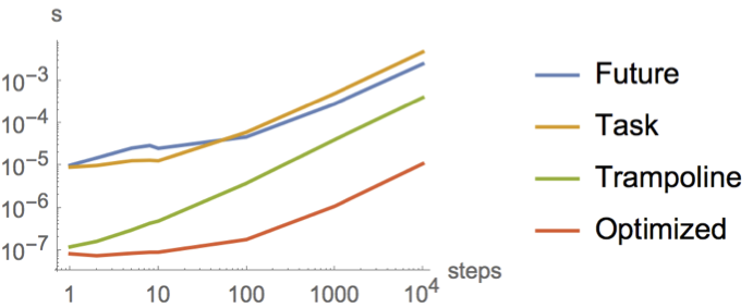
I did some comparisons using Caliper and made this pretty graph for you:

The horizontal axis is the number of steps, and the vertical axis is the mean time that number of steps took over a few thousand runs.

This graph shows that Task is slightly faster than Future for submitting to thread pools (blue and yellow lines marked Future and Task respectively) only for very small tasks; up to about when you get to 50 steps, when (on my Macbook) both futures and tasks cross the 30 μs threshold. This difference is probably due to the fact that a Future is a running computation while a Task is partially constructed up front and explicitly run later. So with the Future the threads might just be waiting for more work. The overhead of Task.run seems to catch up with us at around 50 steps.

But honestly the difference between these two lines is not something I would care about in a real application, because if we jump on the trampoline instead of submitting to a thread pool (green line marked Trampoline), things are between one and two orders of magnitude faster.

If we only jump on the trampoline when we really need it (red line marked Optimized), we can gain another order of magnitude. Compared to the original naïve version that always goes to the thread pool, this is now the difference between running your program on a 10 MHz machine and running it on a 1 GHz machine.

If we measure without using any Task/Future at all, the line tracks the Optimized red line pretty closely then shoots to infinity around 1000 (or however many frames fit in your stack space) because the program crashes at that point.

In summary, if we’re smart about trampolines vs thread pools, Future vs Task, and optimize for our stack size, we can go from milliseconds to microseconds with not very much effort. Or seconds to milliseconds, or weeks to hours, as the case may be.

After giving it a lot of thought I have come to the conclusion that I won’t be involved in “Functional Programming in Java”. There are many reasons, including that I just don’t think I can spend the time to make this a good book. Looking at all the things I have scheduled for the rest of the year, I can’t find the time to work on it.

More depressingly, the thought of spending a year or more writing another book makes me anxious. I know from experience that making a book (at least a good one) is really hard and takes up a lot of mental energy. Maybe one day there will be a book that I will want to forego a year of evenings and weekends for, but today is not that day.

Originally, the content of FPiJ was going to be based on “Functional Programming in Scala”, but after some discussion with the publisher I think we were all beginning to see that this book deserved its own original content specifically on an FP style in Java.

I really do think such a thing deserves its own original book. Since Java is strictly less suitable for functional programming than Scala is, a book on FP in Java will have to lay a lot of groundwork that we didn’t have to do with FPiS, and it will have to forego a lot of the more advanced topics.

I wish the author of that book, and the publisher, all the best and I hope they do well. I’m sorry to let you all down, but I’m sure this is for the best.

Our book, Functional Programming in Scala, relies heavily on exercises. Hints and answers for those exercises are not actually in the book, but are freely available on GitHub under a permissive MIT license. Likewise, we have written chapter notes that we reference throughout the book and made them available as a community-editable wiki.

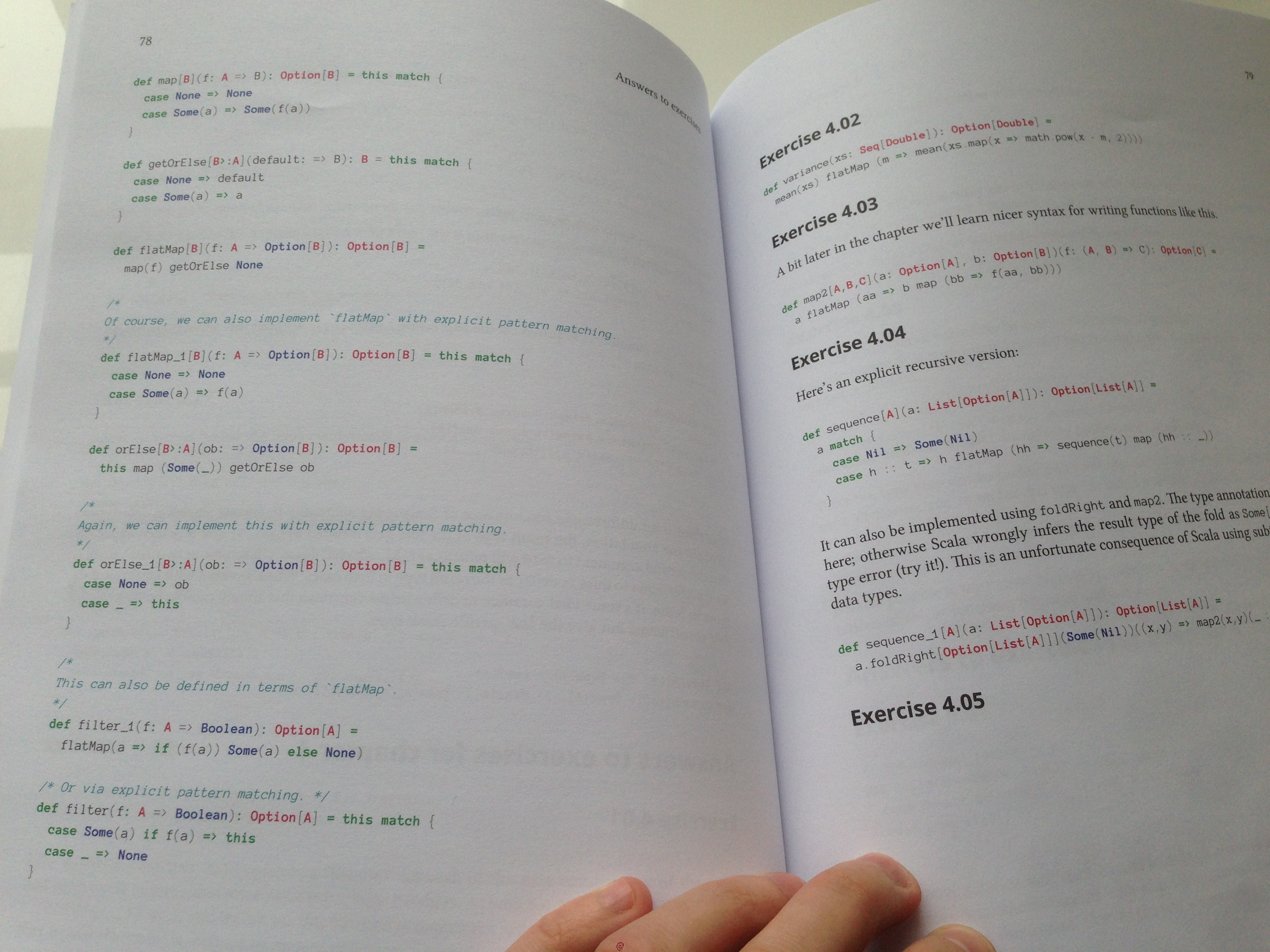
Naturally, readers get the most out of this book by downloading the source code from GitHub and doing the exercises as they read. But a number of readers have made the comment that they wish they could have the hints and answers with them when they read the book on the train to and from work, on a long flight, or wherever there is no internet connection or it’s not convenient to use a computer.

It is of course entirely possible to print out the chapter notes, hints, and exercises, and take them with you either as a hardcopy or as a PDF to use on a phone or tablet. Well, I’ve taken the liberty of doing that work for you. I wrote a little script to concatenate all the chapter notes, errata, hints, and answers into Markdown files and then just printed them all to a single document, tweaking a few things here and there. I’m calling this A companion booklet to “Functional Programming in Scala”. It is released under the same MIT license as the content it aggregates. This means you’re free to copy it, distribute or sell it, or basically do whatever you want with it. The Markdown source of the manuscript is available on my GitHub.

I have made an electronic version of this booklet available on Leanpub as as a PDF, ePub, and Kindle file on a pay-what-you-want basis (minimum of $0.99). It has full color syntax highlighting throughout and a few little tweaks to make it format nicely. The paper size is standard US Letter which makes it easy to print on most color printers. If you choose to buy the booklet from Leanpub, they get a small fee, a small portion of the proceeds goes to support Liberty in North Korea, and the rest goes to yours truly. You’ll also get updates when those inevitably happen.

If you don’t care about any of that, you can grab the PDF from here with my compliments.

The booklet is also available from CreateSpace or Amazon as a full color printed paperback. This comes in a nicely bound glossy cover for just a little more than the price of printing (they print it on demand for you). I’ve ordered one and I’m really happy with the quality of this print:

The print version is of course under the same permissive license, so you can make copies of it, make derivative works, or do whatever you want. It’s important to note that with this booklet I’ve not done anything other than design a little cover and then literally print out this freely available content and upload it to Amazon, which anybody could have done (and you still can if you want).

I hope this makes Functional Programming in Scala more useful and more enjoyable for more people.

Like a lot of people, I keep a list of books I want to read. And because there are a great many more books that interest me than I can possibly read in my lifetime, this list has become quite long.

In the olden days of brick-and-mortar bookstores and libraries, I would discover books to read by browsing shelves and picking up what looked interesting at the time. I might even find something that I knew was on my list. “Oh, I’ve been meaning to read that!”

The Internet changes this dynamic dramatically. It makes it much easier for me to discover books that interest me, and also to access any book that I might want to read, instantly, anywhere. At any given time, I have a couple of books that I’m “currently reading”, and when I finish one I can start another immediately. I use Goodreads to manage my to-read list, and it’s easy for me to scroll through the list and pick out my next book.

But again, this list is very long. So I wanted a good way to filter out books I will really never read, and sort it such that the most “important” books in some sense show up first. Then every time I need a new book I could take the first one from the list and make a binary decision: either “I will read this right now”, or “I am never reading this”. In the latter case, if a book interests me enough at a later time, I’m sure it will find its way back onto my list.

The problem then is to find a good metric by which to rank books. Goodreads lets users rank books with a star-rating from 1 to 5, and presents you with an average rating by which you can sort the list. The problem is that a lot of books that interest me have only one rating and it’s 5 stars, giving the book an “average” of 5.0. So if I go with that method I will be perpetually reading obscure books that one other person has read and loved. This is not necessarily a bad thing, but I do want to branch out a bit.

Another possibility is to use the number of ratings to calculate a confidence interval for the average rating. For example, using the Wilson score I could find an upper and lower bound s1 and s2 (higher and lower than the average rating, respectively) that will let me say “I am 95% sure that any random sample of readers of an equal size would give an average rating between s1 and s2.” I could then sort the list by the lower bound s1.

But this method is dissatisfactory for a number of reasons. First, it’s not clear how to fit star ratings to such a measure. If we do the naive thing and count a 1-star rating as 1/5 and a 5 star rating as 5/5, that counts a 1-star rating as a “partial success” in some sense. We could discard 1-stars as 0, and count 2, 3, 4, and 5 stars as 25%, 50%, 75%, and 100%, respectively.

But even if we did make it fit somehow, it turns out that if you take any moderately popular book on Goodreads at random, it will have an average rating somewhere close to 4. I could manufacture a prior based on this knowledge and use that instead of the normal distribution or the Jeffreys prior in the confidence interval, but that would still not be a very good ranking because reader review metascores are meaningless.

In the article “Reader review metascores are meaningless”, Stephanie Shun suggests using the percentage of 5-star ratings as the relevant metric rather than the average rating. This is a good suggestion, since even a single 5-star rating carries a lot of actionable information whereas an average rating close to 4.0 carries very little.

I can then use the Wilson score directly, counting a 5-star rating as a successful trial and any other rating as a failed one. I can then just use the normal distribution instead of working with an artisanally curated prior.

Mathematica makes it easy to generate the Wilson score. Here, pos is the number of positive trials (number of 5-star ratings), n is the number of total ratings, and confidence is the desired confidence percentage. I’m taking the lower bound of the confidence interval to get my score.

1
2
3
4
5
6
7
8
9
10

Wilson[pos_, n_, confidence_] := 
  If[n == 0 || n < pos, 0, 
    With[{
      z = Quantile[NormalDistribution[], 1 - (1 - confidence)/2], 
      p = pos/n
    },
    (-(z Sqrt[(z^2/(4 n) + (1 - p) p)/n]) + z^2/(2 n) + p) /
      (z^2/n + 1)
    ]
  ]

Now I just need to get the book data from Goodreads. Fortunately, it has a pretty rich API. I just need a developer key, which anyone can get for free.

For example, to get the ratings for a given book id, we can use their XML api for books and pattern match on the result to get the ratings by score:

1
2
3
4
5
6
7
8
9
10

Ratings[id_] := Ratings[id] = 
  With[{
    raw = Cases[Import[ToString[StringForm[
        "http://www.goodreads.com/book/show.xml?key=``&id=``", key, id]]],
      XMLElement["rating_dist", _, {d_}] -> d, Infinity]
  }, 
  With[{
    data = StringSplit[#, ":"] & /@ StringSplit[raw, "|"]
  }, Block[{}, Pause[1];
  FromDigits /@ Association[Rule @@@ First[data]]]]];

Here, key is my Goodreads developer API key, defined elsewhere. I put a Pause[1] in the call since Goodreads throttles API calls so you can’t make more than one call per second to each API endpoint. I’m also memoizing the result, by assigning to Ratings[id] in the global environment.

Ratings will give us an association list with the number of ratings for each score from 1 to 5, together with the total. For example, for the first book in their catalogue, Harry Potter and the Half-Blood Prince, here are the scores:

1
2
3
4
5
6
7
8

In[1]:= Ratings[1]

Out[1]= <|"5"     ->  782740,
          "4"     ->  352725,
          "3"     ->  111068,
          "2"     ->   17693,
          "1"     ->    5289,
          "total" -> 1269515|>

Sweet. Let’s see how Harry Potter #6 would score with our rating:

1
2
3

In[2]:= Wilson[Out[1]["5"], Out[1]["total"], 0.95]

Out[2]= 0.61572

So Wilson is 95% confident that in any random sample of about 1.2 million Harry Potter readers, at least 61.572% of them would give The Half-Blood Prince a 5-star rating. That turns out to be a pretty high score, so if this book were on my list (which it isn’t), it would feature pretty close to the very top.

But now the score for a relatively obscure title is too low. For example, the lower bound of the 95% confidence interval for a single-rating 5-star book will be 0.206549, which will be towards the bottom of any list. This means I would never get to any of the obscure books on my reading list, since they would be edged out by moderately popular books with an average rating close to 4.0.

See, if I’ve picked a book that I want to read, I’d consider five ratings that are all five stars a much stronger signal than the fact that people who like Harry Potter enough to read 5 previous books loved the 6th one. Currently the 5*5 book will score 57%, a bit weaker than the Potter book’s 62%.

I can fix this by lowering the confidence level. Because honestly, I don’t need a high confidence in the ranking. I’d rather err on the side of picking up a deservedly obscure book than to miss out on a rare gem. Experimenting with this a bit, I find that a confidence around 80% raises the obscure books enough to give me an interesting mix. For example, a 5*5 book gets a 75% rank, while the Harry Potter one stays at 62%.

I’m going to call that the Rúnar rank of a given book. The Rúnar rank is defined as the lower bound of the 1-1/q Wilson confidence interval for scoring in the qth q-quantile. In the special case of Goodreads ratings, it’s the 80% confidence for a 5-star rating.

1
2

RunarRank[id_] := With[{ratings = Ratings[id]},
  Wilson[ratings["5"], ratings["total"], .8]]]

Unfortunately, there’s no way to get the rank of all the books in my reading list in one call to the Goodreads API. And when I asked them about it they basically said “you can’t do that”, so I’m assuming that feature will not be added any time soon. So I’ll have to get the reading list first, then call RunarRank for each book’s id. In Goodreads, books are managed by “shelves”, and the API allows getting the contents of a given shelf, 200 books at a time:

1
2
3
4
5
6
7
8
9
10
11
12
13
14
15
16
17
18

GetShelf[user_, shelf_] :=
  With[{raw = 
    Cases[Import[
      ToString[
       StringForm[
        "http://www.goodreads.com/review/list.xml?v=2&key=``&id=``&\
shelf=``&sort=avg_rating&order=d&per_page=200", key, user, shelf]]], 
     XMLElement[
       "book", _, {___, XMLElement["id", ___, {id_}], ___, 
        XMLElement["title", _, {title_}], ___, 
        XMLElement["average_rating", _, {avg_}], ___, 
        XMLElement[
         "authors", _, {XMLElement[
           "author", _, {___, 
            XMLElement[
             "name", _, {author_}], ___}], ___}], ___}] -> {"id" -> 
        id, "title" -> title, "author" -> author, "avg" -> avg}, 
     Infinity]}, Association /@ raw]

I’m doing a bunch of XML pattern matching here to get the id, title, average_rating, and first author of each book. Then I put that in an association list. I’m getting only the top-200 books on the list by average rating (which currently is about half my list).

With that in hand, I can get the contents of my “to-read” shelf with GetShelf[runar, "to-read"], where runar is my Goodreads user id. And given that, I can call RunarRank on each book on the shelf, then sort the result by that rank:

1
2
3

RunarSort[shelf_] :=
 Sort[Map[Function[x, Append[x, "rank" -> RunarRank[x["id"]]]], 
   shelf], #1["rank"] > #2["rank"] &]

To get the ranked reading list of any user:

1

ReadingList[user_] := RunarSort[GetShelf[user, "to-read"]]

And to print it out nicely:

1
2
3
4
5
6
7

Gridify[books_] := 
 Grid[Flatten[
   Cases[books, 
    b_ -> {
      {b["id"], b["title"], UnitConvert[b["rank"], "Percent"]},
      {"", b["author"], b["avg"]}, {"", "", ""} }], 1],
   Alignment -> Left]

Now I can get, say, the first 10 books on my improved reading list:

1

Gridify[ReadingList[runar][[1 ;; 10]]]

I’m quite happy with that. Some very popular and well-loved books interspersed with obscure ones with exclusively (or almost exclusively) positive reviews. The most satisfying thing is that the rating carries a real meaning. It’s basically the relative likelihood that I will enjoy the book enough to rate it five stars.

I can test this ranking against books I’ve already read. Here’s the top of my “read” shelf, according to their Rúnar Rank:

That’s perfect. Those are definitely books I thouroughly enjoyed and would heartily recommend. Especially that last one.

I’ve published this function as a Wolfram Cloud API, and you can call it at https://www.wolframcloud.com/app/objects/4f4a7b3c-38a5-4bf3-81b6-7ca8e05ea100. It takes two URL query parameters, key and user, which are your Goodreads API key and the Goodreads user ID whose reading list you want to generate, respectively. Enjoy!

It’s well known that there is a trade-off in language and systems design between expressiveness and analyzability. That is, the more expressive a language or system is, the less we can reason about it, and vice versa. The more capable the system, the less comprehensible it is.

This principle is very widely applicable, and it’s a useful thing to keep in mind when designing languages and libraries. A practical implication of being aware of this principle is that we always make components exactly as expressive as necessary, but no more. This maximizes the ability of any downstream systems to reason about our components. And dually, for things that we receive or consume, we should require exactly as much analytic power as necessary, and no more. That maximizes the expressive freedom of the upstream components.

I find myself thinking about this principle a lot lately, and seeing it more or less everywhere I look. So I’m seeking a more general statement of it, if such a thing is possible. It seems that more generally than issues of expressivity/analyzability, a restriction at one semantic level translates to freedom and power at another semantic level.

What I want to do here is give a whole bunch of examples. Then we’ll see if we can come up with an integration for them all. This is all written as an exercise in thinking out loud and is not to be taken very seriously.

Examples from computer science

Context-free and regular grammars

In formal language theory, context-free grammars are more expressive than regular grammars. The former can describe strictly more sets of strings than the latter. On the other hand, it’s harder to reason about context-free grammars than regular ones. For example, we can decide whether two regular expressions are equal (they describe the same set of strings), but this is undecidable in general for context-free grammars.

Monads and applicative functors

If we know that an applicative functor is a monad, we gain some expressive power that we don’t get with just an applicative functor. Namely, a monad is an applicative functor with an additional capability: monadic join (or “bind”, or “flatMap”). That is, context-sensitivity, or the ability to bind variables in monadic expressions.

This power comes at a cost. Whereas we can always compose any two applicatives to form a composite applicative, two monads do not in general compose to form a monad. It may be the case that a given monad composes with any other monad, but we need some additional information about it in order to be able to conclude that it does.

Actors and futures

Futures have an algebraic theory, so we can reason about them algebraically. Namely, they form an applicative functor which means that two futures x and y make a composite future that does x and y in parallel. They also compose sequentially since they form a monad.

Actors on the other hand have no algebraic theory and afford no algebraic reasoning of this sort. They are “fire and forget”, so they could potentially do anything at all. This means that actor systems can do strictly more things in more ways than systems composed of futures, but our ability to reason about such systems is drastically diminished.

Typed and untyped programming

When we have an untyped function, it could receive any type of argument and produce any type of output. The implementation is totally unrestricted, so that gives us a great deal of expressive freedom. Such a function can potentially participate in a lot of different expressions that use the function in different ways.

A function of type Bool -> Bool however is highly restricted. Its argument can only be one of two things, and the result can only be one of two things as well. So there are 4 different implementations such a function could possibly have. Therefore this restriction gives us a great deal of analyzability.

For example, since the argument is of type Bool and not Any, the implementation mostly writes itself. We need to consider only two possibilities. Bool (a type of size 2) is fundamentally easier to reason about than Any (a type of potentially infinite size). Similarly, any usage of the function is easy to reason about. A caller can be sure not to call it with arguments other than True or False, and enlist the help of a type system to guarantee that expressions involving the function are meaningful.

Total functional programming

Programming in non-total languages affords us the power of general recursion and “fast and loose reasoning” where we can transition between valid states through potentially invalid ones. The cost is, of course, the halting problem. But more than that, we can no longer be certain that our programs are meaningful, and we lose some algebraic reasoning. For example, consider the following:

1

map (- n) (map (+ n) xs)) == xs

This states that adding n to every number in a list and then subtracting n again should be the identity. But what if n actually throws an exception or never halts? In a non-total language, we need some additional information. Namely, we need to know that n is total.

Referential transparency and side effects

The example above also serves to illustrate the trade-off between purely functional and impure programming. If n could have arbitrary side effects, algebraic reasoning of this sort involving n is totally annihilated. But if we know that n is referentially transparent, algebraic reasoning is preserved. The power of side effects comes at the cost of algebraic reasoning. This price includes loss of compositionality, modularity, parallelizability, and parametricity. Our programs can do strictly more things, but we can conclude strictly fewer things about our programs.

Example from infosec

There is a principle in computer security called The Principle of Least Privilege. It says that a user or program should have exactly as much authority as necessary but no more. This constrains the power of the entity, but greatly enhances the power of others to predict and reason about what the entity is going to do, resulting in the following benefits:

• Compositionality – The fewer privileges a component requires, the easier it is to deploy inside a larger environment. For the purposes of safety, higher privileges are a barrier to composition since a composite system requires the highest privileges of any of its components.
• Modularity – A component with restricted privileges is easier to reason about in the sense that its interaction with other components will be limited. We can reason mechanically about where this limit actually is, which gives us better guarantees about the the security and stability of the overall system. A restricted component is also easier to test in isolation, since it can be run inside an overall restricted environment.

Example from politics

Some might notice an analogy between the Principle of Least Privilege and the idea of a constitutionally limited government. An absolute dictatorship or pure democracy will have absolute power to enact whatever whim strikes the ruler or majority at the moment. But the overall stability, security, and freedom of the people is greatly enhanced by the presence of legal limits on the power of the government. A limited constitutional republic also makes for a better neighbor to other states.

More generally, a ban on the initiation of physical force by one citizen against another, or by the government against citizens, or against other states, makes for a peaceful and prosperous society. The “cost” of such a system is the inability of one person (or even a great number of people) to impose their preferences on others by force.

An example from mathematics

The framework of two-dimensional Euclidean geometry is simply an empty page on which we can construct lines and curves using tools like a compass and straightedge. When we go from that framework to a Cartesian one, we constrain ourselves to reasoning on a grid of pairs of numbers. This is a tradeoff between expressivity and analyzability. When we move fom Euclidean to Cartesian geometry, we lose the ability to assume isotropy of space, intersection of curves, and compatibility between dimensions. But we gain much more powerful things through the restriction: the ability to precisely define geometric objects, to do arithmetic with them, to generalize to higher dimensions, and to reason with higher abstractions like linear algebra and category theory.

Examples from everyday life

Driving on roads

Roads constrain the routes we can take when we drive or walk. We give up moving in a straight line to wherever we want to go. But the benefit is huge. Roads let us get to where we’re going much faster and more safely than we would otherwise.

Commodity components

Let’s say you make a decision to have only one kind of outfit that you wear on a daily basis. You just go out and buy multiple identical outfits. Whereas you have lost the ability to express yourself by the things you wear, you have gained a certain ability to reason about your clothing. The system is also fault-tolerant and compositional!

Summary

What is this principle? Here are some ways of saying it:

• Things that are maximally general for first-order applications are minimally useful for higher-order applications, and vice versa.
• A language that is maximally expressive is minimally analyzable.
• A simplifying assumption at one semantic level paves the way to a richer structure at a higher semantic level.

What do you think? Can you think of a way to integrate these examples into a general principle? Do you have other favorite examples of this principle in action? Is this something everyone already knows about and I’m just late to the party?