Taking a Break From Twitter

Oct 29th, 2014 1:23 pm

Today I disabled my Twitter account. Probably only temporarily, but we’ll see. This is just a quick note to let everyone know that I’m not leaving Twitter because of anything specific. It’s not that you said or did anything wrong. I just find that it’s becoming an energy sink for me. I’m putting Twitter away as a measure to control my focus, and to better control what information I consume and produce.

Hopefully this means that I will post more here when I have something interesting to share. If you need to reach me, I’m available by email. My address is runar at this blog’s domain.

(UPDATE 2014-12-21): I’ve recreated my Twitter account, but I’m now using the service in a different way. The biggest change is that I don’t follow anyone. It’s strictly a broadcasting device for me, and not an information consumption device.

At Long Last

Sep 18th, 2014 1:09 pm

In early September 2014, we published Functional Programming in Scala. It is now available from all major booksellers, and from the publisher at manning.com/bjarnason. It’s available as a beautiful paper book, on Kindle and other e-book readers, and as a PDF file.

I just want to share my personal story of how this book came to exist. A much shorter version of this story became the preface for the finished book, but here is the long version.

Around 2006 I was working in Austin and coming up on my 8th anniversary as an enterprise Java programmer. I had started to notice that I was making a lot of the same mistakes over and over again. I had a copy of the Gang of Four’s Design Patterns on my desk that I referred to frequently, and I built what I thought were elegant object-oriented designs. Every new project started out well enough, but became a big ball of mud after a while. My once-elegant class hierarchies gathered bugs, technical debt, and unimplemented features. Making changes started to feel like trudging through a swamp. I was never confident that I wasn’t introducing defects as I went. My code was difficult to test or reuse, and impossible to reason about. My productivity plummeted, and a complete rewrite became inevitable. It was a vicious cycle.

In looking for a more disciplined approach, I came across Haskell and functional programming. Here was a community of people with a sound methodology for reasoning about their programs. In other words, they actually knew what they were doing. I found a lot of good ideas and proceeded to import them to Java. A little later I met Tony Morris, who had been doing the same, on IRC. He told me about this new JVM language, Scala. Tony had a library called Scalaz (scala-zed) that made FP in Scala more pleasant, and I started contributing to that library. One of the other people contributing to Scalaz was Paul Chiusano, who was working for a company in Boston. In 2008 he invited me to come work with him, doing Scala full time. I sold my house and everything in it, and moved to Boston.

Paul co-organized the Boston Area Scala Enthusiasts, a group that met monthly at Google’s office in Cambridge. It was a popular group, mainly among Java programmers who were looking for something better. But there was a clear gap between those who had come to Scala from an FP perspective and those who saw Scala as just a better way to write Java. In April 2010 another of the co-organizers, Nermin Serifovic, said he thought there was “tremendous demand” for a book that would bridge that gap, on the topic of functional programming in Scala. He suggested that Paul and I write that book. We had a very clear idea of the kind of book we wanted to write, and we thought it would be quick and easy. More than four years later, I think we have made a good book.

Paul and I hope to convey in this book some of the excitement that we felt when we were first discovering FP. It’s encouraging and empowering to finally feel like we’re writing comprehensible software that we can reuse and confidently build upon. We want to invite you to the world of programming as it could be and ought to be.

– Rúnar Óli Bjarnason

Boston, August 2014

Monoid Morphisms, Products, and Coproducts

Mar 19th, 2014 12:00 am

Today I want to talk about relationships between monoids. These can be useful to think about when we’re developing libraries involving monoids, and we want to express some algebraic laws among them. We can then check these with automated tests, or indeed prove them with algebraic reasoning.

This post kind of fell together when writing notes on chapter 10, “Monoids”, of Functional Programming in Scala. I am putting it here so I can reference it from the chapter notes at the end of the book.

Monoid homomorphisms

Let’s take the String concatenation and Int addition as example monoids that have a relationship. Note that if we take the length of two strings and add them up, this is the same as concatenating those two strings and taking the length of the combined string:

(a.length + b.length) == (a + b).length

So every String maps to a corresponding Int (its length), and every concatenation of strings maps to the addition of corresponding lengths.

The length function maps from String to Int while preserving the monoid structure. Such a function, that maps from one monoid to another in such a preserving way, is called a monoid homomorphism. In general, for monoids M and N, a homomorphism f: M => N, and all values x:M, y:M, the following equations hold:

f(x |+| y) == (f(x) |+| f(y))

f(mzero[M]) == mzero[N]

The |+| syntax is from Scalaz and is obtained by importing scalaz.syntax.monoid._. It just references the append method on the Monoid[T] instance, where T is the type of the arguments. The mzero[T] function is also from that same import and references zero in Monoid[T].

This homomorphism law can have real practical benefits. Imagine for example a “result set” monoid that tracks the locations of a particular set of records in a database or file. This could be as simple as a Set of locations. Concatenating several thousand files and then proceeding to search through them is going to be much slower than searching through the files individually and then concatenating the result sets. Particularly since we can potentially search the files in parallel. A good automated test for our result set monoid would be that it admits a homomorphism from the data file monoid.

Monoid isomorphisms

Sometimes there will be a homomorphism in both directions between two monoids. If these are inverses of one another, then this kind of relationship is called a monoid isomorphism and we say that the two monoids are isomorphic. More precisely, we will have two monoids A and B, and homomorphisms f: A => B and g: B => A. If f(g(b)) == b and g(f(a)) == a, for all a:A and b:B then f and g form an isomorphism.

For example, the String and List[Char] monoids with concatenation are isomorphic. We can convert a String to a List[Char], preserving the monoid structure, and go back again to the exact same String we started with. This is also true in the inverse direction, so the isomorphism holds.

Other examples include (Boolean, &&) and (Boolean, ||) which are isomorphic via not.

Note that there are monoids with homomorphisms in both directions between them that nevertheless are not isomorphic. For example, (Int, *) and (Int, +). These are homomorphic to one another, but not isomorphic (thanks, Robbie Gates).

Monoid products and coproducts

If A and B are monoids, then (A,B) is certainly a monoid, called their product:

def product[A:Monoid,B:Monoid]: Monoid[(A, B)] =
  new Monoid[(A, B)] {
    def append(x: (A, B), y: => (A, B)) =
      (x._1 |+| y._1, x._2 |+| y._2)
    val zero = (mzero[A], mzero[B])
  }

But is there such a thing as a monoid coproduct? Could we just use Either[A,B] for monoids A and B? What would be the zero of such a monoid? And what would be the value of Left(a) |+| Right(b)? We could certainly choose an arbitrary rule, and we may even be able to satisfy the monoid laws, but would that mean we have a monoid coproduct?

To answer this, we need to know the precise meaning of product and coproduct. These come straight from Wikipedia, with a little help from Cale Gibbard.

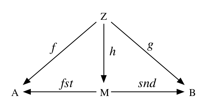
A product M of two monoids A and B is a monoid such that there exist homomorphisms fst: M => A, snd: M => B, and for any monoid Z and morphisms f: Z => A and g: Z => B there has to be a unique homomorphism h: Z => M such that fst(h(z)) == f(z) and snd(h(z)) == g(z) for all z:Z. In other words, the following diagram must commute:

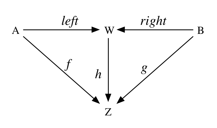
A coproduct W of two monoids A and B is the same except the arrows are reversed. It’s a monoid such that there exist homomorphisms left: A => W, right: B => W, and for any monoid Z and morphisms f: A => Z and g: B => Z there has to be a unique homomorphism h: W => Z such that h(left(a)) == f(a) and h(right(b)) == g(b) for all a:A and all b:B. In other words, the following diagram must commute:

We can easily show that our productMonoid above really is a monoid product. The homomorphisms are the methods _1 and _2 on Tuple2. They simply map every element of (A,B) to a corresponding element in A and B. The monoid structure is preserved because:

(p |+| q)._1 == (p._1 |+| q._1)
(p |+| q)._2 == (p._2 |+| q._2)

zero[(A,B)]._1 == zero[A]
zero[(A,B)]._2 == zero[B]

And for any other monoid Z, and morphisms f: Z => A and g: Z => B, we can construct a unique morphism from Z to (A,B):

def factor[A:Monoid,B:Monoid,Z:Monoid](z: Z)(f: Z => A, g: Z => B): (A, B) =
  (f(z), g(z))

And this really is a homomorphism because we just inherit the homomorphism law from f and g.

What does a coproduct then look like? Well, it’s going to be a type C[A,B] together with an instance coproduct[A:Monoid,B:Monoid]:Monoid[C[A,B]]. It will be equipped with two monoid homomorphisms, left: A => C[A,B] and right: B => C[A,B] that satisfy the following (according to the monoid homomorphism law):

(left(a1) |+| left(a2)) == left(a1 |+| a2)
(right(b1) |+| right(b2)) == right(b1 |+| b2)

left[A,B](mzero[A]) == mzero[C[A,B]]
right[A,B](mzero[B]) == mzero[C[A,B]]

And additionally, for any other monoid Z and homomorphisms f: A => Z and g: B => Z we must be able to construct a unique homomorphism from C[A,B] to Z:

def fold[A:Monoid,B:Monoid,Z:Monoid](c: C[A,B])(f: A => Z, g: B => Z): Z

Right off the bat, we know some things that definitely won’t work. Just using Either is a non-starter because there’s no well-defined zero for it, and there’s no way of appending a Left to a Right. But what if we just added that structure?

Free monoids on coproducts

The underlying set of a monoid A is just the type A without the monoid structure. The coproduct of types A and B is the type Either[A,B]. Having “forgotten” the monoid structure of both A and B, we can recover it by generating a free monoid on Either[A,B], which is just List[Either[A,B]]. The append operation of this monoid is list concatenation, and the identity for it is the empty list.

Clearly List[Either[A,B]] is a monoid, but does it permit a homomorphism from both monoids A and B? If so, then the following properties should hold:

List(Left(a1)) ++ List(Left(a2))) == List(Left(a1 |+| a2))
List(Right(b1)) ++ List(Right(b2))) == List(Right(b1 |+| b2))

They clearly do not hold! The lists on the left of == will have two elements and the lists on the right will have one element. Can we do something about this?

Well, the fact is that List[Either[A,B]] is not exactly the monoid coproduct of A and B. It’s still “too big”. The problem is that we can observe the internal structure of expressions.

What we need is not exactly the List monoid, but a new monoid called the free monoid product:

sealed class Eithers[A:Monoid,B:Monoid](
  private val toList: List[Either[A,B]]) {

    def ++(p: Eithers[A,B]): Eithers[A,B] =
      Eithers(toList ++ p.toList)

    def fold[Z:Monoid](f: A => Z, g: B => Z): Z =
      toList.foldRight(mzero[Z]) {
        case (Left(a), z) => f(a) |+| z
        case (Right(b), z) => g(b) |+| z
      }
}

object Eithers {
  def left[A:Monoid,B:Monoid](a: A): Eithers[A,B] =
    Eithers(List(Left(a)))
  def right[A:Monoid,B:Monoid](b: B): Eithers[A,B] =
    Eithers(List(Right(b)))

  def empty[A:Monoid,B:Monoid]: Eithers[A,B] = new Eithers(Nil)

  def apply[A:Monoid,B:Monoid](xs: List[Either[A,B]]): Eithers[A,B] =
    new Eithers(xs.foldRight(List[Either[A,B]]()) {
      case (Left(a1), Left(a2) :: xs) => Left(a1 |+| a2) :: xs
      case (Right(b1), Right(b2) :: xs) => Right(b1 |+| b2) :: xs
      case (e, xs) => e :: xs
    })
}

Eithers[A,B] is a kind of List[Either[A,B]] that has been normalized so that consecutive As and consecutive Bs have been collapsed using their respective monoids. So it will contain alternating A and B values.

The only remaining problem is that a list full of identities is not exactly the same as the empty list. Remember the unit part of the homomorphism law:

Eithers(List(Left(mzero))) == Eithers.empty
Eithers(List(Right(mzero))) == Eithers.empty

This doesn’t hold at the moment. As Cale Gibbard points out in the comments below, Eithers is really the free monoid on the coproduct of semigroups A and B.

We could check each element as part of the normalization step to see if it equals(zero) for the given monoid. But that’s a problem, as there are lots of monoids for which we can’t write an equals method. For example, for the Int => Int monoid (with composition), we must make use of a notion like extensional equality, which we can’t reasonably write in Scala.

So what we have to do is sort of wave our hands and say that equality on Eithers[A,B] is defined as whatever notion of equality we have for A and B respectively, with the rule that es.fold[(A,B)] defines the equality of Eithers[A,B]. For example, for monoids that really can have Equal instances:

def eithersEqual[A:Monoid:Equal,B:Monoid:Equal] =
  new Equal[Eithers[A,B]] {
    def equal(xs: Eithers[A,B], ys: Eithers[A,B]) = {
      def le(a: A): (A,B) = (a, mzero[B])
      def ri(b: B): (A,B) = (mzero[A], b)
      def z(es: Eithers[A,B]): (A,B) =
        es.fold(le, ri)(Monoid[(A,B)])

      z(xs) === z(ys)
    }
  }

So we have to settle with a list full of zeroes being “morally equivalent” to an empty list. The difference is observable in e.g. the time it takes to traverse the list.

Setting that issue aside, Eithers is a monoid coproduct because it permits monoid homomorphisms from A and B:

Eithers(List(Left(a1))) ++ Eithers(List(Left(a2)))) ==
  Eithers(List(Left(a1 |+| a2)))
Eithers(List(Right(b1))) ++ Eithers(List(Right(b2)))) ==
  Eithers(List(Right(b1 |+| b2)))

And fold really is a homomorphism, and we can prove it by case analysis. Here’s the law again:

(e1.fold(f,g) |+| e2.fold(f,g)) == (e1 ++ e2).fold(f,g)

If either of e1 or e2 is empty then the result is the fold of the other, so those cases are trivial. If they are both nonempty, then they will have one of these forms:

e1 = [..., Left(a1)]
e2 = [Left(a2), ...]

e1 = [..., Right(b1)]
e2 = [Right(b2), ...]

e1 = [..., Left(a)]
e2 = [Right(b), ...]

e1 = [..., Right(b)]
e2 = [Left(a), ...]

In the first two cases, on the right of the == sign in the law, we perform a1 |+| a2 and b1 |+| b2 respectively before concatenating. In the other two cases we simply concatenate the lists. The ++ method on Eithers takes care of doing this correctly for us. On the left of the == sign we fold the lists individually and they will be alternating applications of f and g. So then this law amounts to the fact that f(a1 |+| a2) == f(a1) |+| f(a2) in the first case, and the same for g in the second case. In the latter two cases this amounts to a homomorphism on List. So as long as f and g are homomorphisms, so is _.fold(f,g). Therefore, Eithers[A,B] is a coproduct of A and B.

Free Monads and the Yoneda Lemma

Nov 1st, 2013 12:00 am

Last week I gave a talk on Purely Functional I/O at Scala.io in Paris. The slides for the talk are available here. In it I presented a data type for IO that is supposedly a “free monad”. But the monad I presented is not exactly the same as scalaz.Free and some people have been asking me why there is a difference and what that difference means.

IO as an application of Free

The Free monad in Scalaz is given a bit like this:

sealed trait Free[F[_],A]
case class Return[F[_],A](a: A) extends Free[F,A]
case class Suspend[F[_],A](s: F[Free[F, A]]) extends Free[F,A]

And throughout the methods on Free, it is required that F is a functor because in order to get at the recursive step inside a Suspend, we need to map over the F somehow.

But the IO monad I gave in the talk looks more like this:

sealed trait IO[F[_],A]
case class Return[F[_],A](a: A) extends IO[F,A]
case class Req[F[_],I,A](req: F[I], k: I => IO[F,A]) extends IO[F,A]

And it could actually be stated as an application of Free:

type IO[F[_],A] = Free[({type λ[α] = (F[I], I => α) forSome {type I}})#λ, A]

So in a very superficial sense, this is how the IO monad relates to Free. The monad IO[F,_] for a given F is the free monad generated by the functor (F[I], I => _) for some type I. And do note that this is a functor no matter what F is.

IO as equivalent to Free

There is a deeper sense in which IO and Free are actually equivalent (more precisely, isomorphic). That is, there exists a transformation from one to the other and back again. Since the only difference between IO and Free is in the functors F[_] vs ∃I. (F[I], I => _), we just have to show that these two are isomorphic for any F.

The Yoneda lemma

There is an important result in category theory known as the Yoneda lemma. What it says is that if you have a function defined like this…

def map[B](f: A => B): F[B]

…then you certainly have a value of type F[A]. All you need is to pass the identity function to map in order to get the value of type F[A] out of this function. In fact, a function like this is in practice probably defined as a method on a value of type F[A] anyway. This also means that F is definitely a functor.

The Yoneda lemma says that this goes the other way around as well. If you have a value of type F[A] for any functor F and any type A, then you certainly have a map function with the signature above.

In scala terms, we can capture this in a type:

trait Yoneda[F[_], A] {
  def map[B](f: A => B): F[B]
}

And the Yoneda lemma says that there is an isomorphism between Yoneda[F,A] and F[A], for any functor F and any type A. Here is the proof:

import scalaz._

def toYo[F[_]:Functor,A](fa: F[A]) = new Yoneda[F,A] {
  def map[B](f: A => B) = Functor[F].map(fa)(f)
}

def froYo[F[_],A](yo: Yoneda[F,A]) = yo.map(a => a)

CoYoneda

Of course, this also means that if we have a type B, a function of type (B => A) for some type A, and a value of type F[B] for some functor F, then we certainly have a value of type F[A]. This is kind of obvious, since we can just pass the B => A and the F[B] to the map function for the functor and get our F[A].

But the opposite is also true, and that is the really interesting part. If we have a value of type F[A], for any F and A, then we can always destructure it into a value of type F[B] and a function of type B => A, at least for some type B. And it turns out that we can do this even if F is not a functor.

This is the permutation of the Yoneda lemma that we were using in IO above. That is, IO[F, A] is really Free[({type λ[α] = CoYoneda[F,α]})#λ, A], given:

trait CoYoneda[F[_], A] {
  type I
  def f: I => A
  def fi: F[I]
}

And the lemma says that CoYoneda[F,A] is isomorphic to F[A]. Here is the proof:

def toCoYo[F[_],A](fa: F[A]) = new CoYoneda[F,A] {
  type I = A
  val f = (a: A) => a
  val fi = fa
}
def froCoYo[F[_]:Functor,A](yo: CoYo) = Functor[F].map(yo.fi)(yo.f)

Of course, this destructuring into CoYoneda using the identity function is the simplest and most general, but there may be others for specific F and A depending on what we know about them.

So there you have it. The scalaz.Free monad with its Suspend(F[Free[F,A]]) constructor and the IO monad with its Req(F[I], I => IO[F,A]) constructor are actually equivalent. The latter is simply making use of CoYoneda to say the same thing.

Why bother? The useful part is that CoYoneda[F,_] is a functor for any F, so it’s handy to use in a free monad since we can then drop the requirement that F is a functor. What’s more, it gives us map fusion for free, since map over CoYoneda is literally just function composition on its f component. Although this latter is, in the absence of tail call elimination, not as useful as it could be in Scala.

I hope that sheds a little bit of light on the Yoneda lemma as well as the different embeddings of free monads.

Free Monoids and Free Monads

Aug 20th, 2013 12:00 am

In a series of old posts, I once talked about the link between lists and monoids, as well as monoids and monads. Now I want to talk a little bit more about monoids and monads from the perspective of free structures.

List is a free monoid. That is, for any given type A, List[A] is a monoid, with list concatenation as the operation and the empty list as the identity element.

def freeMonoid[A]: Monoid[List[A]] = new Monoid[List[A]] {
  def unit = Nil
  def op(a1: List[A], a2: List[A]) = a1 ++ a2
}

Being a free monoid means that it’s the minimal such structure. List[A] has exactly enough structure so that it is a monoid for any given A, and it has no further structure. This also means that for any given monoid B, there must exist a transformation, a monoid homomorphism from List[A] to B:

def foldMap[A,B:Monoid](as: List[A])(f: A => B): B

Given a mapping from A to a monoid B, we can collapse a value in the monoid List[A] to a value in B.

Free monads

Now, if you followed my old posts, you already know that monads are “higher-kinded monoids”. A monoid in a category where the objects are type constructors (functors, actually) and the arrows between them are natural transformations. As a reminder, a natural transformation from F to G can be represented this way in Scala:

trait ~>[F[_],G[_]] {
  def apply[A](a: F[A]): G[A]
}

And it turns out that there is a free monad for any given functor F:

sealed trait Free[F[_],A]
case class Return[F[_],A](a: A) extends Free[F,A]
case class Suspend[F[_],A](f: F[Free[F,A]]) extends Free[F,A]

Analogous to how a List[A] is either Nil (the empty list) or a product of a head element and tail list, a value of type Free[F,A] is either an A or a product of F[_] and Free[F,_]. It is a recursive structure. And indeed, it has exactly enough structure to be a monad, for any given F, and no more.

When I say “product” of two functors like F[_] and Free[F,_], I mean a product like this:

trait :*:[F[_],G[_]] {
  type λ[A] = F[G[A]]
}

So we might expect that there is a monad homomorphism from a free monad on F to any monad that F can be transformed to. And indeed, it turns out that there is. The free monad catamorphism is in fact a monad homomorphism. Given a natural transformation from F to G, we can collapse a Free[F,A] to G[A], just like with foldMap when given a function from A to B we could collapse a List[A] to B.

def runFree[F[_],G[_]:Monad,A](as: Free[F,A])(f: F ~> G): G[A]

But what’s the equivalent of foldRight for Free? Remember, foldRight takes a unit element z and a function that accumulates into B so that B doesn’t actually have to be a monoid. Here, f is a lot like the monoid operation, except it takes the current A on the left:

def foldRight[A,B](as: List[A])(z: B)(f: (A, B) => B): B

The equivalent for Free takes a natural transformation as its unit element, which for a monad happens to be monadic unit. Then it takes a natural transformation as its f argument, that looks a lot like monadic join, except it takes the current F on the left:

type Id[A] = A

def foldFree[F[_]:Functor,G[_],A](
  as: Free[F,A])(
  z: Id ~> G)(
  f: (F:*:G)#λ ~> G): G[A]

In this case, G does not have to be a monad at all.

Free as well as natural transformations and product types are available in Scalaz.

Machines and Stream Processing

Jan 26th, 2013 12:34 pm

I gave a talk on “Machines” and stream processing in Haskell and Scala, to the Brisbane Functional Programming Group at Microsoft HQ in December 2012. A lot of people have asked me for the slides, so here they are:

Machines.pdf

The preëmptive answer to the usual follow-up question is that the talk was not recorded.

What Purity Is and Isn’t

Sep 13th, 2012 10:07 pm

A lot of discussion about “purity” goes on without participants necessarily having a clear idea of what it means exactly. Such discussion is generally unhelpful and distracting.

What purity is

The typical definition of purity (and the one we use in our book) goes something like this:

An expression e is referentially transparent if for all programs p, every occurrence of e in p can be replaced with the result of evaluating e without changing the result of evaluating p.

A function f is pure if the expression f(x) is referentially transparent for all referentially transparent x.

Now, something needs to be made clear right up front. Like all definitions, this holds in a specific context. In particular, the context needs to specify what “evaluating” means. It also needs to define “program”, “occurrence”, and the semantics of “replacing” one thing with another.

In a programming language like Haskell, Java, or Scala, this context is pretty well established. The process of evaluation is a reduction to some normal form such as weak head or beta normal form.

A simple example

To illustrate, let’s consider programs in an exceedingly simple language that we will call Sigma. An expression in Sigma has one of the following forms:

A literal character string like "a", "foo", "", etc.
A concatenation, s + t, for expressions s and t.
A special Ext expression that denotes input from an external source.

Now, without an evaluator for Sigma, it is a purely abstract algebra. So let’s define a straigtforward evaluator eval for it, with the following rules:

A literal string is already in normal form.
eval(s + t) first evaluates s and t and concatenates the results into one literal string.
eval(Ext) reads a line from standard input and returns it as a literal string.

This might seem very simple, but it is still not clear whether Ext is referentially transparent with regard to eval. It depends. What does “reads a line” mean, and what is “standard input” exactly? This is all part of a context that needs to be established.

Here’s one implementation of an evaluator for Sigma, in Scala:

sealed trait Sigma
case class Lit(s: String) extends Sigma
case class Concat(s: Sigma, t: Sigma) extends Sigma
case object Ext extends Sigma

def eval1(sig: Sigma): Sigma = sig match {
  case Concat(s, t) => {
    val Lit(e1) = eval1(s)
    val Lit(e2) = eval1(t)
    Lit(e1 + e2)
  }
  case Ext => Lit(readLine)
  case x => x
}

Now, it’s easy to see that the Ext instruction is not referentially transparent with regard to eval1. Replacing Ext with eval1(ext) does not preserve meaning. Consider this:

val x = Ext
eval1(Concat(x, x))

VS this:

val x = eval1(Ext)
eval1(Concat(x, x))

That’s clearly not the same thing. The former will get two strings from standard input and concatenate them together. The latter will get only one string, store it as x, and return x + x.

Now consider a slightly different evaluator:

def eval2(sig: Sigma, stdin: String): Sigma = sig match {
  case Concat(s, t) => {
    val Lit(e1) = eval2(s, stdin)
    val Lit(e2) = eval2(t, stdin)
    Lit(e1 + e2)
  }
  case Ext => Lit(stdin)
  case x => x
}

In this case, the Ext instruction clearly is referentially transparent with regard to eval2, because our standard input is just a string, and it is always the same string. So you see, the purity of functions in the Sigma language very much depends on how that language is interpreted.

This is the reason why Haskell programs are considered “pure”, even in the presence of IO. A value of type IO a in Haskell is simply a function. Reducing it to normal form (evaluating it) has no effect. An IO action is of course not referentially transparent with regard to unsafePerformIO, but as long as your program does not use that it remains a referentially transparent expression.

What purity is not

In my experience there are more or less two camps into which unhelpful views on purity fall.

The first view, which we will call the empiricist view, is typically taken by people who understand “pure” as a pretentious term, meant to denegrate regular everyday programming as being somehow “impure” or “unclean”. They see purity as being “academic”, detached from reality, in an ivory tower, or the like.

This view is premised on a superficial understanding of purity. The assumption is that purity is somehow about the absence of I/O, or not mutating memory. But how could any programs be written that don’t change the state of memory? At the end of the day, you have to update the CPU’s registers, write to memory, and produce output on a display. A program has to make the computer do something, right? So aren’t we just pretending that our programs don’t run on real computers? Isn’t it all just an academic exercise in making the CPU warm?

Well, no. That’s not what purity means. Purity is not about the absence of program behaviors like I/O or mutable memory. It’s about delimiting such behavior in a specific way.

The other view, which I will call the rationalist view, is typically taken by people with overexposure to modern analytic philosophy. Expressions are to be understood by their denotation, not by reference to any evaluator. Then of course every expression is really referentially transparent, and so purity is a distinction without a difference. After all, an imperative side-effectful C program can have the same denotation as a monadic, side-effect-free Haskell program. There is nothing wrong with this viewpoint, but it’s not instructive in this context. Sure, when designing in the abstract, we can think denotationally without regard to evaluation. But when concretizing the design in terms of an actual programming language, we do need to be aware of how we expect evaluation to take place. And only then are referential transparency and purity useful concepts.

Both of these, the rationalist and empiricist views, conflate different levels of abstraction. A program written in a programming language is not the same thing as the physical machine that it may run on. Nor is it the same thing as the abstractions that capture its meaning.

New Beginnings

Sep 4th, 2012 1:29 am

I have not seriously updated the old Apocalisp blog for quite some time. Mostly this is due to the fact that I have been spending all of my creative time outside of work on writing a book. It’s also partly that putting a post up on WordPress is a chore. It’s like building a ship in a bottle.

So I have decided to make posting really easy for myself by hosting the blog on GitHub. I am using a dead-simple markdown-based framework called Octopress. With this setup I can very easily write a new post from my command line and publish by pushing to GitHub. This is already part of my normal coding workflow, so it feels more friction-free.

The new blog is simply titled “Higher Order”, and is available at blog.higher-order.com. Check back soon for posts that I’ve been sitting on but have been too ~~lazy~~ busy to post.

All of the old content and comments will still be available at the old address, and I’ll probably cross-post to both places for a little while.

Scalaz Tutorial: Enumeration-based I/O With Iteratees

Oct 14th, 2010 12:00 am

Scalaz 5.0 adds an implementation of a concept called Iteratee. This is a highly flexible programming technique for writing enumeration-based input processors that can be freely composed.

A lot of people have asked me to write a tutorial on how this works, specifically on how it is implemented in Scalaz and how to be productive with it, so here we go.

The implementation in Scalaz is based on an excellent article by John W. Lato called “Iteratee: Teaching an Old Fold New Tricks”. As a consequence, this post is also based on that article, and because I am too unoriginal to come up with my own examples, the examples are directly translated from it. The article gives code examples in Haskell, but we will use Scala here throughout.

Motivation

Most programmers have come across the problem of treating an I/O data source (such as a file or a socket) as a data structure. This is a common thing to want to do. To contrast, the usual means of reading, say, a file, is to open it, get a cursor into the file (such as a FileReader or an InputStream), and read the contents of the file as it is being processed. You must of course handle IO exceptions and remember to close the file when you are done. The problem with this approach is that it is not modular. Functions written in this way are performing one-off side-effects. And as we know, side-effects do not compose.

Treating the stream of inputs as an enumeration is therefore desirable. It at least holds the lure of modularity, since we would be able to treat a File, from which we’re reading values, in the same way that we would treat an ordinary List of values, for example.

A naive approach to this is to use iterators, or rather, Iterables. This is akin to the way that you would typically read a file in something like Ruby or Python. Basically you treat it as a collection of Strings:

def getContents(fileName: String): Iterable[String] = {
  val fr = new BufferedReader(new FileReader(fileName))
  new Iterable[String] {
    def iterator = new Iterator[String] {
      def hasNext = line != null
      def next = {
        val retVal = line
        line = getLine
        retVal
      }
      def getLine = {
        var line:String = null
        try {
          line = fr.readLine
        } catch {
          case _ => line = null
        }
        line
      }
      var line = getLine
    }
  }
}

What this is doing is a kind of lazy I/O. Nothing is read from the file until it is requested, and we only hold one line in memory at a time. But there are some serious issues with this approach. It’s not clear when you should close the file handle, or whose responsibility that is. You could have the Iterator close the file when it has read the last line, but what if you only want to read part of the file? Clearly this approach is not sufficient. There are some things we can do to make this more sophisticated, but only at the expense of breaking the illusion that the file really is a collection of Strings.

The Idea

Any functional programmer worth their salt should be thinking right about now: “Instead of getting Strings out of the file, just pass in a function that will serve as a handler for each new line!” Bingo. This is in fact the plot with Iteratees. Instead of implementing an interface from which we request Strings by pulling, we’re going to give an implementation of an interface that can receive Strings by pushing.

And indeed, this idea is nothing new. This is exactly what we do when we fold a list:

def foldLeft[B](b: B)(f: (B, A) => B): B

The second argument is exactly that, a handler for each element in the list, along with a means of combining it with the accumulated value so far.

Now, there are two issues with an ordinary fold that prevent it from being useful when enumerating file contents. Firstly, there is no way of indicating that the fold should stop early. Secondly, a list is held all in memory at the same time.

The Iteratee Solution

Scalaz defines the following two data structures (actual implementation may differ, but this serves for illustration):

trait Input[+E]
case class El[E](e: E) extends Input[E]
case object Empty extends Input[Nothing]
case object EOF extends Input[Nothing]

trait IterV[E,A] {
  def run: A = ... // Implementation omitted
}
case class Done[E,A](a: A, e: Input[E]) extends IterV[E,A]
case class Cont[E,A](k: Input[E] => IterV[E,A]) extends IterV[E,A]

So an input to an iteratee is represented by Input[E], where E is the element type of the input source. It can be either an element (the next element in the file or stream), or it’s one of two signals: Empty or EOF. The Empty signal tells the iteratee that there is not an element available, but to expect more elements later. The EOF signal tells the iteratee that there are no more elements to be had.

Note that this particular set of signals is kind of arbitrary. It just facilitates a particular set of use cases. There’s no reason you couldn’t have other signals for other use cases. For example, a signal I can think of off the top of my head would be Restart, which would tell the iteratee to start its result from scratch at the current position in the input.

IterV[E,A] represents a computation that can be in one of two states. It can be Done, in which case it will hold a result (the accumulated value) of type A. Or it can be waiting for more input of type E, in which case it will hold a continuation that accepts the next input.

Let’s see how we would use this to process a List. The following function takes a list and an iteratee and feeds the list’s elements to the iteratee.

def enumerate[E,A]: (List[E], IterV[E,A]) => IterV[E,A] = {
  case (Nil, i) => i
  case (_, i@Done(_, _)) => i
  case (x :: xs, Cont(k)) => enumerate(xs, k(El(x)))
}

Now let’s see some actual iteratees. As a simple example, here is an iteratee that counts the number of elements it has seen:

def counter[A]: IterV[A,Int] = {
  def step(n: Int): Input[A] => IterV[A,Int] = {
    case El(x) => Cont(step(n + 1))
    case Empty => Cont(step(n))
    case EOF => Done(n, EOF)
  }
  Cont(step(0))
}

And here’s an iteratee that discards the first n elements:

def drop[E,A](n: Int): IterV[E,Unit] = {
  def step: Input[E] => IterV[E,Unit] = {
    case El(x) => drop(n - 1)
    case Empty => Cont(step)
    case EOF => Done((), EOF)
  }
  if (n == 0) Done((), Empty) else Cont(step)
}

And one that takes the first element from the input:

def head[E]: IterV[E, Option[E]] = {
  def step: Input[E] => IterV[E, Option[E]] = {
    case El(x) => Done(Some(x), Empty)
    case Empty => Cont(step)
    case EOF => Done(None, EOF)
  }
  Cont(step)
}

Let’s go through this code. Each one defines a “step” function, which is the function that will handle the next input. Each one starts the iteratee in the Cont state, and the step function always returns a new iteratee in the next state based on the input received. Note in the last one (head), we are using the Empty signal to indicate that we want to remove the element from the input. The utility of this will be clear when we start composing iteratees.

Now, an example usage. To get the length of a list, we write:

val length: Int = enumerate(List(1,2,3), counter[Int]).run // 3

The run method on IterV just gets the accumulated value out of the Done iteratee. If it isn’t done, it sends the EOF signal to itself first and then gets the value.

Composing Iteratees

Notice a couple of things here. With iteratees, the input source can send the signal that it has finished producing values. And on the other side, the iteratee itself can signal to the input source that it has finished consuming values. So on one hand, we can leave an iteratee “running” by not sending it the EOF signal, so we can compose two input sources and feed them into the same iteratee. On the other hand, an iteratee can signal that it’s done, at which point we can start sending any remaining elements to another iteratee. In other words, iteratees compose sequentially.

In fact, IterV[E,A] is an instance of the Monad type class for each fixed E, and composition is very similar to the way monadic parsers compose:

def flatMap[B](f: A => IterV[E,B]) = this match {
  case Done(x, e) => f(x) match {
    case Done(y, _) => Done(y, e)
    case Cont(k) => k(e)
  }
  case Cont(k) => Cont(e => k(e) flatMap f)
}

Here then is an example of composing iteratees with a for-comprehension:

def drop1Keep1[E]: IterV[E, Option[E]] = for {
  _ <- drop(1)
  x <- head
} yield x

The iteratee above discards the first element it sees and returns the second one. The iteratee below does this n times, accumulating the kept elements into a list.

def alternates[E](n: Int): IterV[E, List[E]] =
  drop1Keep1[E].
    replicate[List](n).
    foldRight(Done(List[Option[E]](),Empty))((x, y) => for {
      h <- x
      t <- y
    } yield h :: t).map(_.flatten)

Here’s an example run:

scala> enumerate(List.range(1,15), alternates[Int](5)).run
res85: List[Int] = List(2, 4, 6, 8, 10)

File Input With Iteratees

Using the iteratees to read from file input turns out to be incredibly easy. The only difference is in how the data source is enumerated, and in order to remain lazy (and not prematurely perform any side-effects), we must return our iteratee in a monad:

def enumReader[A](r: BufferedReader,
                  it: IterV[String, A]): IO[IterV[String, A]] = {
  def loop: IterV[String, A] => IO[IterV[String, A]] = {
    case i@Done(_, _) => IO { i }
    case i@Cont(k) => for {
      s <- IO { r.readLine }
      a <- if (s == null) IO { i } else loop(k(El(s)))
    } yield a
  }
  loop(it)
}

The monad being used here is an IO monad that I’ll explain in a second. The important thing to note is that the iteratee is completely oblivious to the fact that it’s being fed lines from a BufferedReader rather than a List.

Here is the IO monad I’m using. As you can see, it’s really just a lazy identity monad:

object io {
  sealed trait IO[A] {
    def unsafePerformIO: A
  }

  object IO {
    def apply[A](a: => A): IO[A] = new IO[A] {
      def unsafePerformIO = a
    }
  }

  implicit val IOMonad = new Monad[IO] {
    def pure[A](a: => A): IO[A] = IO(a)
    def bind[A,B](a: IO[A], f: A => IO[B]): IO[B] = IO {
      implicitly[Monad[Function0]].bind(
        () => a.unsafePerformIO,
        (x:A) => () => f(x).unsafePerformIO)()
    }
  }
}

To read lines from a file, we’ll do something like this:

def bufferFile(f: File) = IO {
  new BufferedReader(new FileReader(f))
}

def closeReader(r: Reader) = IO {
  r.close
}

def bracket[A,B,C](init: IO[A],
                   fin: A => IO[B],
                   body: A => IO[C]): IO[C] =
for { a <- init
      c <- body(a)
      _ <- fin(a) }
  yield c

def enumFile[A](f: File, i: IterV[String, A]): IO[IterV[String, A]] =
  bracket(bufferFile(f),
          closeReader(_:BufferedReader),
          enumReader(_:BufferedReader, i))

The enumFile method uses bracketing to ensure that the file always gets closed. It’s completely lazy though, so nothing actually happens until you call unsafePerformIO on the resulting IO action:

scala> enumFile(new File("/Users/runar/Documents/Iteratees.txt"), head) map (_.run)                
res2: io.IO[Option[String]] = io$IO@5f90b584

scala> res2.unsafePerformIO
res3: Option[String] = Some(Scalaz Tutorial: Enumeration-Based I/O With Iteratees)

That uses the “head” iteratee from above to get the first line of the file that I’m using to edit this blog post.

We can get the number of lines in two files combined, by composing two enumerations and using our “counter” iteratee from above:

def lengthOfTwoFiles(f1: File, f2: File): IO[Int] = for {
  l1 <- enumFile(f1, counter)
  l2 <- enumFile(f2, l1)
} yield l2.run

So what we have here is a uniform and compositional interface for enumerating both pure and effectful data sources. We can avoid holding on to the entire input in memory when we don’t want to, and we have complete control over when to stop iterating. The iteratee can decide whether to consume elements, leave them intact, or even truncate the input. The enumerator can decide whether to shut the iteratee down by sending it the EOF signal, or to leave it open for other enumerators.

There is even more to this approach, as we can use iteratees not just to read from data sources, but also to write to them. That will have to await another post.

Structural Pattern Matching in Java

Aug 21st, 2009 12:00 am

(updated for Java 8)

One of the great features of modern programming languages is structural pattern matching on algebraic data types. Once you’ve used this feature, you don’t ever want to program without it. You will find this in languages like Haskell and Scala.

In Scala, algebraic types are provided by case classes. For example:

sealed trait Tree
case object Empty extends Tree
case class Leaf(n: Int) extends Tree
case class Node(l: Tree, r: Tree) extends Tree

To define operations over this algebraic data type, we use pattern matching on its structure:

def depth(t: Tree): Int = t match {
  case Empty => 0
  case Leaf(n) => 1
  case Node(l, r) => 1 + max(depth(l), depth(r))
}

When I go back to a programming language like, say, Java, I find myself wanting this feature. Unfortunately, algebraic data types aren’t provided in Java. However, a great many hacks have been invented over the years to emulate it, knowingly or not.

The Ugly: Interpreter and Visitor

What I have used most throughout my career to emulate pattern matching in languages that lack it are a couple of hoary old hacks. These venerable and well respected practises are a pair of design patterns from the GoF book: Interpreter and Visitor.

The Interpreter pattern really does describe an algebraic structure, and it provides a method of reducing (interpreting) the structure. However, there are a couple of problems with it. The interpretation is coupled to the structure, with a “context” passed from term to term, and each term must know how to mutate the context appropriately. That’s minus one point for tight coupling, and minus one for relying on mutation.

The Visitor pattern addresses the former of these concerns. Given an algebraic structure, we can define an interface with one “visit” method per type of term, and have each term accept a visitor object that implements this interface, passing it along to the subterms. This decouples the interpretation from the structure, but still relies on mutation. Minus one point for mutation, and minus one for the fact that Visitor is incredibly crufty. For example, to get the depth of our tree structure above, we have to implement a TreeDepthVisitor. A good IDE that generates boilerplate for you is definitely recommended if you take this approach.

On the plus side, both of these patterns provide some enforcement of the exhaustiveness of the pattern match. For example, if you add a new term type, the Interpreter pattern will enforce that you implement the interpretation method. For Visitor, as long as you remember to add a visitation method for the new term type to the visitor interface, you will be forced to update your implementations accordingly.

The Bad: Instanceof

An obvious approach that’s often sneered at is runtime type discovery. A quick and dirty way to match on types is to simply check for the type at runtime and cast:

public static int depth(Tree t) {
  if (t instanceof Empty)
    return 0;
  if (t instanceof Leaf)
    return 1;
  if (t instanceof Node)
    return 1 + max(depth(((Node) t).left), depth(((Node) t).right));
  throw new RuntimeException("Inexhaustive pattern match on Tree.");
}

There are some obvious problems with this approach. For one thing, it bypasses the type system, so you lose any static guarantees that it’s correct. And there’s no enforcement of the exhaustiveness of the matching. But on the plus side, it’s both fast and terse.

The Good: Functional Style

There are at least two approaches that we can take to approximate pattern matching in Java more closely than the above methods. Both involve utilising parametric polymorphism and functional style. Let’s consider them in order of increasing preference, i.e. less preferred method first.

Safe and Terse - Disjoint Union Types

The first approach is based on the insight that algebraic data types represent a disjoint union of types. Now, if you’ve done any amount of programming in Java with generics, you will have come across (or invented) the simple pair type, which is a conjunction of two types:

public abstract class P2<A, B> {
  public A _1();
  public B _2();
}

A value of this type can only be created if you have both a value of type A and a value of type B. So (conceptually, at least) it has a single constructor that takes two values. The disjunction of two types is a similar idea, except that a value of type Either<A, B> can be constructed with either a value of type A or a value of type B:

public final class Either<A, B> {
  ...
  public static <A, B> Either<A, B> left(A a) { ... }
  public static <A, B> Either<A, B> right(B a) { ... }
  ...
}

Encoded as a disjoint union type, then, our Tree data type above is: Either<Empty, Either<Leaf, Node>>

Let’s see that in context. Here’s the code.

public abstract class Tree {
  // Constructor private so the type is sealed.
  private Tree() {}

  public abstract Either<Empty, Either<Leaf, Node>> toEither();

  public static final class Empty extends Tree {
    public <T> T toEither() {
      return left(this);
    }

    public Empty() {}
  }

  public static final class Leaf extends Tree {
    public final int n;

    public Either<Empty, Either<Leaf, Node>> toEither() {
      return right(Either.<Leaf, Node>left(this));
    }

    public Leaf(int n) { this.n = n; }
  }

  public static final class Node extends Tree {
    public final Tree left;
    public final Tree right;

    public Either<Empty, Either<Leaf, Node>> toEither() {
      return right(Either.<Leaf, Node>right(this));
    }

    public Node(Tree left, Tree right) {
      this.left = left; this.right = right;
    }
  }
}

The neat thing is that Either<A, B> can be made to return both Iterable<A> and Iterable<B> in methods right() and left(), respectively. One of them will be empty and the other will have exactly one element. So our pattern matching function will look like this:

public int depth(Tree t) {
  Either<Empty, Either<Leaf, Node>> eln = t.toEither();
  for (Empty e: eln.left())
    return 0;
  for (Either<Leaf, Node> ln: eln.right()) {
    for (leaf: ln.left())
      return 1;
    for (node: ln.right())
      return 1 + max(depth(node.left), depth(node.right));
  }
  throw new RuntimeException("Inexhaustive pattern match on Tree.");
}

That’s terse and readable, as well as type-safe. The only issue with this is that the exhaustiveness of the patterns is not enforced, so we’re still only discovering that error at runtime. So it’s not all that much of an improvement over the instanceof approach.

Safe and Exhaustive: Church Encoding

Alonzo Church was a pretty cool guy. Having invented the lambda calculus, he discovered that you could encode data in it. We’ve all heard that every data type can be defined in terms of the kinds of operations that it supports. Well, what Church discovered is much more profound than that. A data type IS a function. In other words, an algebraic data type is not just a structure together with an algebra that collapses the structure. The algebra IS the structure.

Consider the boolean type. It is a disjoint union of True and False. What kinds of operations does this support? Well, you might want to do one thing if it’s True, and another if it’s False. Just like with our Tree, where we wanted to do one thing if it’s a Leaf, and another thing if it’s a Node, etc.

But it turns out that the boolean type IS the condition function. Consider the Church encoding of booleans:

true  = λa.λb.a
false = λa.λb.b

So a boolean is actually a binary function. Given two terms, a boolean will yield the former term if it’s true, and the latter term if it’s false. What does this mean for our Tree type? It too is a function:

empty = λa.λb.λc.a
leaf  = λa.λb.λc.λx.b x
node  = λa.λb.λc.λl.λr.c l r

You can see that this gives you pattern matching for free. The Tree type is a function that takes three arguments:

A value to yield if the tree is empty. A unary function to apply to an integer if it’s a leaf. A binary function to apply to the left and right subtrees if it’s a node. The type of such a function looks like this (Scala notation):

T => (Int => T) => (Tree => Tree => T) => T

Or equivalently:

(Empty => T) => (Leaf => T) => (Node => T) => T

Translated to Java, we need this method on Tree:

public abstract <T> T match(Function<Empty, T> a,
                            Function<Leaf, T> b,
                            Function<Node, T> c);

The Function interface is in the java.util package in Java 8, but you can definitely make it yourself in previous versions:

public interface Function<A, B> { public B apply(A a); }

Now our Tree code looks like this:

public abstract class Tree {
  // Constructor private so the type is sealed.
  private Tree() {}

  public abstract <T> T match(Function<Empty, T> a,
                              Function<Leaf, T> b,
                              Function<Node, T> c);

  public static final class Empty extends Tree {
    public <T> T match(Function<Empty, T> a,
                       Funciton<Leaf, T> b,
                       Function<Node, T> c) {
      return a.apply(this);
    }

    public Empty() {}
  }

  public static final class Leaf extends Tree {
    public final int n;

    public <T> T match(Function<Empty, T> a,
                       Function<Leaf, T> b,
                       Function<Node, T> c) {
      return b.apply(this);
    }

    public Leaf(int n) { this.n = n; }
  }

  public static final class Node extends Tree {
    public final Tree left;
    public final Tree right;

    public <T> T match(Function<Empty, T> a,
                       Function<Leaf, T> b,
                       Function<Node, T> c) {
      return c.apply(this);
    }

    public Node(Tree left, Tree right) {
      this.left = left; this.right = right;
    }
  }
}

And we can do our pattern matching on the calling side:

public int depth(Tree t) {
  return t.match((Empty e) -> 0,
                 (Leaf l) -> 1,
                 (Node n) -> 1 + max(depth(n.left), depth(n.right));
}

This is almost as terse as the Scala code, and very easy to understand. Everything is checked by the type system, and we are guaranteed that our patterns are exhaustive. This is an ideal solution.

Conclusion

With some slightly clever use of generics and a little help from our friends Church and Curry, we can indeed emulate structural pattern matching over algebraic data types in Java, to the point where it’s almost as nice as a built-in language feature.

So throw away your Visitors and set fire to your GoF book.

← Older Blog Archives Newer →

Higher Order

Philosophy and functional programming.